Dynamic Delta Hedging – Extending the Monte Carlo simulation model to Put contracts

October 29, 2012 by jawwad·Comments Off

Dynamic Delta Hedging – Monte Carlo Simulation in Excel for hedging European put contracts

In our previous post on Dynamic Delta Hedging for European Call Options we built a simple simulation in model in Excel that simulated an underlying price series and a step by step trace of a Dynamic Delta Hedging simulation for a call option.

In this post we will modify and extend the model for European Put options. The basic approach remains the same but a simple modification is required to make the sheet work for European Put contracts.

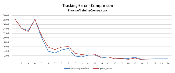
Figure 1 Delta Hedging – Put Options – Monte Carlo Simulation

The end result would be a dynamic simulation graphical output showing the original option value and the replicating portfolio that is created to hedge it.

If you remember, our Dynamic Delta Hedging strategy for Call Options relied on going long (buying) Delta x S and financing this purchase by borrowing the difference between our purchase and the premium received for writing the option. This strategy defined the structure of our Monte Carlo Simulation spread sheet in Excel.

Figure 2 Delta Hedging – The baseline model and simulated values

Delta Hedge – Put Options – Tweaking the original Monte Carlo Simulation model

How would you change this model for hedging a European put contract?

In a call option the probability of exercise goes up as the underlying price goes up. For a put option the opposite is true. For a call option as the probability of exercise goes up, we buy portions of the underlying to hedge our exposure and manage our dollar cost average purchase price.

For a put option therefore we short more of the underlying as probability of exercise goes up ( the probability is N(d2) for a Call, N(-d2) for a Put) and vice versa when the probability goes down.

For a call because we are short cash we borrow it to finance our purchases. For a put option the short sale of the underlying generates cash and we invest the proceeds for the duration that we remain short.

Therefore the structure of our dynamic delta hedging sheet for a European put contract changes and becomes:

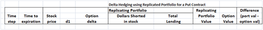
Figure 3 Dynamic Delta Hedging – Baseline model for European put options

The only difference are:

a) In the replicating portfolio: Where we are now short Delta x S and have lent the proceeds from the short sale

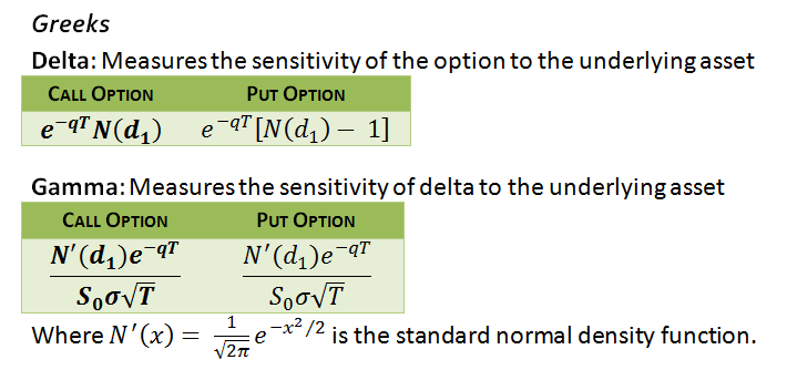
b) Option Delta calculation where we are using N(d1) – 1 rather than N(d1) as the option delta for a put option.

As per our earlier model we still need to simulate:

a) The underlying stock price

b) Option Delta for a put option linked to the underlying stock price

c) Replicating portfolio comprised of a short position in Delta x S (Spot price of stock) and a long position in Borrowing B.

d) Difference between the replicating portfolio and the option value to calculate tracking error.

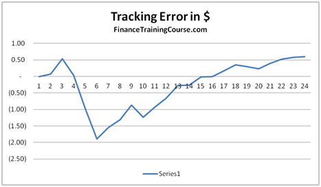
Figure 4 Delta Hedging – Put Options – Tracking Error

If you are unfamiliar Monte Carlo Simulation please see the Monte Caro Simulation Training Guide below as well as our posts on Monte Carlo simulation before proceeding further.

We use Barclays Bank and assume that the bank will pay no dividends over the life of the option.

Delta Hedging Model using Monte Carlo Simulations – Assumptions

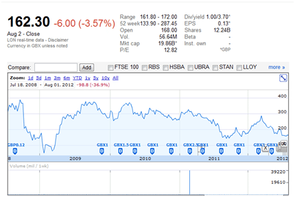
Figure 5 Dynamic Delta Hedging – Barclays bank price chart

Delta Hedge – Put Contract – Simulating the underlying using Monte Carlo Simulation

We will assume that the spot price is 162.3, the strike price 150, the daily volatility will range between 2.5% to 5%. Implied annualized volatility will be assumed to be 40%. Risk free rate of interest will be 1%, time to maturity will be one year. As discussed above, the stock will pay no dividends.

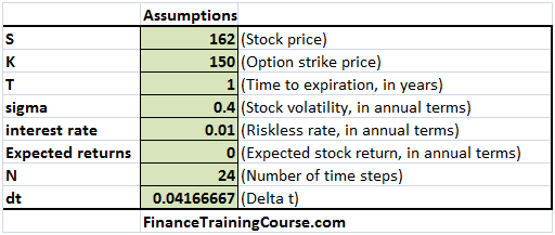
Figure 6 Delta Hedging – Key Assumptions

Using the above assumptions simulate a path of Barclays share price over the next one year. For each value of the underlying stock price we also calculate d1 using the standard Black Scholes European option pricing.

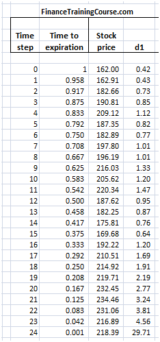
Figure 7 Delta Hedging – Put Option – Simulating the underlying

The actual stock price simulation with the original discrete formula and the Excel implementation is shown below and is the same as the approach used earlier for Delta Hedging. The only difference is that our Delta Hedging sheet worked with a 12 step forecast. For put options we are using a 24 step simulation.

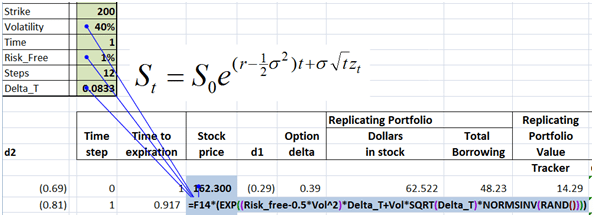
Figure 8 Delta Hedging – Simulating the underlying

Armed with d1 we can now calculate option delta as well as the value of the replicating portfolio (Short Delta x S + Total lending).

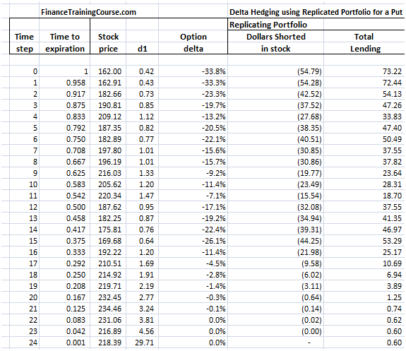
Figure 9 Delta Hedging – Put Option – Completing the Picture

Delta Hedge – Put Contract – Calculating the amount lent for each time step

The dollars shorted calculation is simple (Delta x S), it is the total lending calculation that requires some attention.

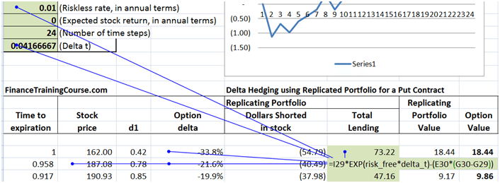
Figure 10 Delta Hedging – Put Option – Calculating Amount lent

The calculation at time step one is simple. We receive $18.44 in premium. Our short position generates $54.79 in cash. The total cash available is 73.22. We immediately lend it at the risk free rate. But what happens at step two in the image above. Price jump to $187.08 and our delta falls to -21.6% from -33.8%. Our short position declines from $54.79 to $40.49. Where does the approximately $14 change comes from?

The original balance at time 1 has grown at the risk free rate for the time step in question (one time step). However the incremental change in stock is given by the change in Delta (G30 – G29) times the new underlying stock price. The way the formula is structured is such that it will release cash when the stock price rises (Put Delta gets less negative) and consume cash when prices decline (Put Delta get more negative).

Put Option – Delta Hedging – Putting the rest of the sheet together

The rest is exactly the same as before. The replicating portfolio is given by (-Delta x S + Amount lent). The option value is calculated by the standard Black Scholes Put Option premium calculation.

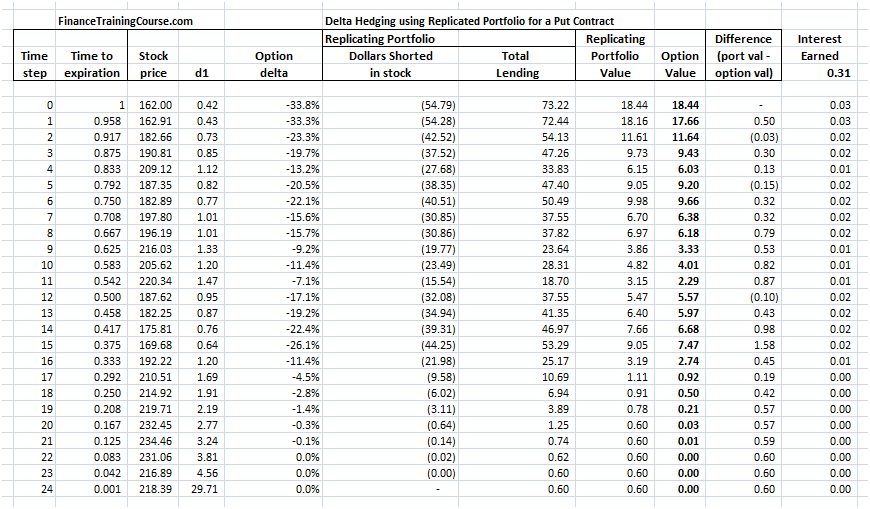
Figure 11 Delta Hedging – Put Option – Total Spreadsheet view

Win a copy of Risk Frameworks & Applications by subscribing – 1 copy for every 10th subscriber

October 28, 2012 by jawwad·Comments Off

Join our subscription list on Face Book and enter your email address in a draw to win selected copies of Risk Frameworks and Applications.

The Funnies – October 2012 Edition

October 27, 2012 by jawwad·Comments Off

That’s it. Can no longer call these Finance funnies. Our selection for the last few months and the next few months will remain distincly political as the world focuses on the upcoming US election. And apparrently so does the creative talent in our time zones. Atleast the theme in this months selection touches foreign policy and gender inquality issues.

An interesting side comment: If cartoons and the funny pages were anything to go by, President Obama has won the election and Mitt is toast. It was the other way round in April, May, June, July & August when the Democrats campaign was just bleeding all over the funny pages. Not so in October 2012, two weeks before the ballot. You can clearly see a distinct shift towards the man from Chicago. Just check the earlier Finance Funnies posts for May, June, July, Aug & September in the related post sections at the end of this post.

We will find out mid November. Till then, enjoy.

The free risk & treasury online training resource guide – popular posts

October 23, 2012 by uzma·Comments Off

Risk & Treasury training resource guide

Here is a list of free resources covering risk and treasury training available on FinanceTrainingCourse.com. They include:

The Advance Risk Management Course

Based on the RM-I & RM-II courses taught at the SP Jain campus in Dubai and Singapore.

Free Risk & Treasury Case studies.

Sample cases, exams, solved solutions & weekend quant challenges.

Risk & Treasury model building course in Excel

Two separate themes that focus on treasury pricing and risk management models in Excel

Asset Liability Management (ALM) Training Guide

Treasury Risk Training Course – Two new courses available online

October 2, 2012 by jawwad·Comments Off

Treasury Risk Training Online Resources

The Treasury Risk Training Course

Two new online & free course reference sites are now up at the following links

The Advance Treasury Risk Management Course Page

The Introduction to Risk Management Course Page

Sample Exam – Treasury Risk Management – Past Final Exam

The two treasury risk training courses were taught as sequential courses to SP Jain GMBA students in Dubai in summer 2012 over two weeks as part of the Financial Risk Management elective series. The Advance course focused on Excel model building using Treasury risk training themes covered earlier in the introductory course. The introductory course used foundation building materials from Value at Risk, ALM and Treasury Risk Management.

The objective was to mix and match treasury risk management frameworks, case studies and hands on risk model building exercises in Excel. The final exam (see practice past examination question above) focused on a real life treasury risk case study from the Margin Risk Management world. Where ever possible we used real treasury risk management case studies and data to ensure students developed a strong sense of what it takes to actually implemented treasury risk management models in practice.

Course content covers topics from the following core risk management themes:

Introduction to Treasury Risk Management
Introduction to Value at Risk – Framework and case studies
Introduction to Delta and Higher Order Hedging for an Options Book
Asset Liability Management – Framework and case studies
Probability of Default models using Merton’s structured approach for FI Analysis
Capital Adequacy & Bank Regulation

Suggested training course instruction time is 36 hours spread over 12 days of classes with 3 hours per day. The outline and the course material require a heavy reading and in class modeling load and are not recommended for the light hearted.

While the first three themes in the course focused on Treasury Risk Management, the last 3 balanced the course material out by introducing credit risk (probability of default models for FI and counter party limit setting), Asset Liability Management (ALM) and Capital Adequacy analysis.

If you would like us to run either of the two course as an in-house workshop at your bank or treasury risk unit please drop me a line at jawwad at the rate alchemya dot com.

Practice Exam Test Question: Pricing and MTM of Interest Rate Swaps (IRS) – Partial solution

September 23, 2012 by jawwad·Comments Off

Practice Exam Test Question – Pricing and MTM of Interest Rate Swaps (IRS)

And now for the last and final part of our Practice Exam Test Question series on Pricing Interest Rate Swaps (IRS). In our first post we walked through the process of building a annualized forward curve and then extending it to semiannual rates.

In this post we will take the forward curve generated in the previous post and use it answer our Interest Rate Swaps (swap rate) and mark to market (valuation) questions.

Here is the projected zero and forward rates curve from our previous post, posted here for convenience. Before you proceed further please take a quick look at the interest rate swap pricing free study guide to review our approach and methodology.

Mark to Market and Valuing an Interest Rate Swap – Practice Test Question and Partial solution

A client has recently entered into a 4.5 year floating rate loan for US$ 400,000,000? The loan will be effective six months from now and will use the following repayment schedule.

Figure 1 Practice Exam Question – Notional Principal for pricing Interest Rate Swaps

The client has asked for a quote for the an effective interest rate risk hedge that would offset the risk of rising interest rates.

a)
What would be the swap rate at cost or breakeven basis for this structure?

b) Would the client be paying fixed or receiving fixed

c) What would be the swap rate if the loan starts at time 2.5 with 10,000,000 and ends at time 3 with an outstanding principal of 10 million.

Here is the output from our solution Excel Sheet. The approach is as per interest rate swap pricing free study guide. The projected forward rates are as per the results above and were driven in the projected forward rates using bootstrapping post. As you can see that the trick here was recognizing that we didn’t have a normal interest rate swap but a forward starting amortizing swap and then adjust the pricing approach accordingly.

a) The exact breakeven swap rate is 13.718% and the breakeven value of each leg (fixed and floating) is 3.001609
million.

b) Since the client is hedging a floating rate loan with this swap he will be paying a fixed rate and receiving the floating rate or simply paying fixed.

Figure 2 The practice test question solution – the interest rate swap pricing, MTM and valuation grid

c) This question is asking you to price a one step FRA or a Forward Rate Agreement. To solve it you should pick the row corresponding to tenor 2.5 and solve for a fixed rate that allows the present value of fixed and floating payments to completely offset each other. This fixed rate is 17.5732%. If you understood the question intuitively you should be able to answer it without resorting to the below solution by simply looking at the applicable forward rate and using that as the breakeven rate.

Figure 3 The practice test question – the FRA pricing, MTM and valuation grid

Common Interest Rate Swap pricing and valuation mistakes made by students in this question

Not making the forward pricing adjustment for the forward starting interest rate swap
Not using the correct notional amount. A number of students used a flat value of 400 million rather than the amortization schedule shared with the question above. Use the correct amortization schedule
Not adjusting for the day count in the fixed as well as floating cash flows. Students often use the full rate when calculating semiannual payment, where as they should be using 180/360 or 182/365 * the relevant interest to account for the fact that the payment is a semiannual interest payment.
Not using the correct applicable floating (forward rate)

d) Six month later the interest rates term structure has changed as shown below. Taking the original Swap structure and assuming that the Swap was purchased at the original breakeven Swap rate, what is the MTM (Mark to Market value of the Swap).

Figure 4 Practice Exam question – Revised Interest Rate Yield Curve

This question requires a simple re-application of the above process one more time. Here are the revised projected forward rates

Figure 5 Revised projected forward rates

The trick now is to remember that we have all moved 6 months forward in time and the IRS is effective now. Based on this assumption this is how the revised grid looks like. The IRS has a negative MTM because we had expected rates to go up and they have actually come down.

Figure 6 Pricing, MTM, Valuing the IRS under the new term structure and yield curve

Once again the biggest mistake students made here was not moving forward in time and pricing the IRS on an as is basis. The second biggest mistake was not using the updated curve and the old Swap Rate calculated from the earlier part of the question.

Practice Test Exam Question and Solution – Bootstrapping Zero and Forward Curves Case Study

September 23, 2012 by jawwad·Comments Off

Practice Test Exam Question Solution for Pricing Interest Rate Swaps – MBA course Derivatives I & II

Here is abbreviated partial solved solution to the practice exam question posed earlier. The practice exam question was used in Derivatives Pricing course taught to MBA students earlier in August 2012. The solution is presented in two parts. The first part of the solution focuses on the bootstrapping zero and forward curve part of the exam. The second part of the solution walks through the actual IRS pricing exercise. This post covers the first partial solution.

The practice exam question had three parts and hence the solution to the practice test question will also be presented in three parts. Before you proceed further please take a quick look at our free interest rate swaps pricing guide. We will only present the basic outputs from the solved solution sheet. You will need to review the interest rate swaps pricing study note to actually build the sheet yourself on your laptop.

Practice Test Exam Question Solution – A review of solution approach

Practice Test Part I dealt with build and plotting Zero and Forward curve using the data given and the bootstrapping approach applied on the given interest rate yield curve given below. The original yield curve was a 5 step curve that gave 5 annualized rates for 5 years.

Figure 1 Practice Exam Question – Given Interest Rate Yield Curve

Practice Test Part II dealt with using the given zero and forward curves to price an Interest Rate Swap (IRS) and calculate the swap rate. The trick was extending the original curve to the new 10 step, semi annual yield curve implied by the 10 step notional amortization schedule given below.

Figure 2 Practice Test Question – The notional amortization schedule

Practice Test Part III dealt with marking to market (MTMing) the interest rate swap for an updated curve a few months later. Once again the trick is to extend the 5 step curve to a 10 step semi-annual curve which can then be used for pricing the interest rate swap.

Figure 3 Practice Test Question – the revised interest rate yield curve

Practice Test Exam Question Solution – Pricing Interest Rate Swap – Part I – Building the Forward Curve

The first step is to break the individual bonds down to their annual cash flows and treat each cash flow as an individual zero coupon bond as explained in the interest rate swap pricing study guide. The output from the first forward curve building step is shown below

Figure 4 Practice Test Question – Solution – Breaking the bonds down to individual cash flows

The second step is to use the individual zero coupon cash flows to boot strap the present value of the principal cash flow at maturity for each of the par bonds as explained in the interest rate swap pricing study guide. The output from the boot strapping step is shown below.

Figure 5 Practice Test Question – Bootstrapping discount factors

The third step is to apply the zero curve and forward curve formula to calculate the relevant zero and forward rates from the table above. As explained in the interest rate swap pricing study note. The output from the zero and forward rate calculation step is shown below.

The final and forth step is to plot the Par, Forward and Zero rates in the required graphical format using MS Excel built in graphic tools.

Figure 6 Practice Test Question – Plot of Par, Zero and Forward curves

Most students make it to this stage without any incident. Some however apply the wrong formula and end up with inconsistent results. If you are not happy with the results just apply a simple calculation cross check. If you calculate the relevant accumulation factors for each given year using your calculated Par, Zero and Forward curves they should all result in the same values as shown below.

The Par Curve Accumulation factor was already calculated above. For the Zero curve the accumulation factor is (1 + zero rate) raised to (compounding period). The accumulation factor for the forward curve is a similarly recursive calculation. Calculate the accumulation factor using the forward curve for the first year. Then use that in your calculation for calculating the accumulation factor using the forward curve for the second year.

If you see a value in the error term row, you have made a mistake in the calculations above. Review and check them.

Figure 7 Practice Test Question – Calculation Cross Check

We have now successfully completed the first part of the test question. We now move on to part II.

Practice Test Exam Question Solution – Pricing Interest Rate Swap – Part II – Extending the Forward Curve

The second part of the question requires us to use the interest rate yield curve above to price a 10 step, semiannual interest rate swap. And this is where confusion reigned supreme.

Step One – Interpolated semiannual yields

We first need to break the original annual yields to maturity down into interpolated semiannual yields as shown below

Figure 8 Practice Test Question – Interpolated semiannual yields.

Then using the same sequence of steps above we break the new implied semiannual bonds down to their zero coupon components, boot strap the curve, calculate the rates and plot the graphs.

Step Two – Zero Coupon Bonds

Figure 9 Practice Test Question – Zero Coupon Bonds by tenor

Step Three – Bootstrapped Discounted Cash Flows for Zeros

Figure 10 Practice Test Question – Bootstrapped Discounted Cash Flows

Step Four – Periodic and Annualized Par, Zero and Forward Rates

Figure 11 Practice Test Question – Model Output – Par, Zero and Forward Rates

Common Mistakes in Part II of the Test Exam

The most common mistakes that killed points for students in the second part of the practice test and exam questions were:

a) Not calculating the interpolated semiannual yields and using the original 5 annualized yield to price the 10 step interest rate swap

b) As a result of (a) above building a 5 x 5 or a 5 x 10 grid versus a 10 x 10 grid as shows in step two and step three above

c) Using annual rates rather than period rates in the 5 x 10 and 10 x 10 grid. Periodic rates are annualized rates divided by 2 since the coupon on the underlying loan is paid semi annually

d) Using periodic rates but then not annualizing them before using them in the IRS pricing later on in Part III of the practice test exam.

The correct solution and required graphical presentation if you didn’t suffer from mistake (a), (b), (c) and (d) above would look like this:

We continue our coverage of this exam question in our next post.

Pricing Interest Rate Swaps – The actual Final Exam question in full

Here is the original post that presented the question earlier today.

I teach the Derivative Pricing and Risk Management courses to EMBA and MBA students in Dubai and Singapore. In a recent exam one question caused a lot of heart ache and pain in exam takers. While most student understood the gist of the question, they still made a number of small mistakes that cost them valuable points in the final score.

If you have an interest rate swap pricing exam or test coming up, here is the solved solution that you can use as a practice exam or practice test question. For best results, first try the exam and the practice and test question and then work through the solution. Best of luck.

Pricing Interest Rate Swaps – Practice Exam – Test prep question

You are given the following term structure of interest rates for US$ using Yield to Maturity (YTM) of Par bonds that pay interest on a semi-annual basis

Figure 12 Test Prep – Practice Exam – The Interest Rates Yield Curve

Using these Par Bond Yields please answer the following questions:

7. Plot the following graph shown in Figure 1 using the above term structure and assuming that that coupon/interest is paid on a Semi Annual basis. This implies that you would need to build a 10 x 10 grid at semi-annual intervals for 5 years. Your graphical plot will show projected rates at 10 points at 10 half years. (15 Points)

Figure 13 Practice Exam – Sample Par, Zero & Forward curve plot

Please see the next page for question number 8

8. A client has recently entered into a 4.5 year floating rate loan for US$ 400,000,000? The loan will be effective six months from now and will use the following repayment schedule. (35 points)

Figure 14 Practice Exam Question – Notional Principal for pricing Interest Rate Swaps

The client has asked for a quote for the an effective interest rate risk hedge that would offset the risk of rising interest rates.

a)
What would be the swap rate at cost or breakeven basis for this structure?

b) Would the client be paying fixed or receiving fixed

c) What would be the swap rate if the loan starts at time 2.5 with 10,000,000 and ends at time 3 with an outstanding principal of 10 million.

Figure 15 Practice Exam question – Revised Interest Rate Yield Curve

Pricing Interest Rate Swaps – Derivative pricing final exam question for practice exams & test prep

September 23, 2012 by jawwad·Comments Off

Pricing Interest Rate Swaps – Final Exam question for test prep

If you have an interest rate swap pricing exam or test coming up, here is the sample question that you can use as a practice exam or practice test question. If you detailed hands on model building interviews for your Sales & Trading, FICC or Risk Management desks, the question has a few twists that can reveal how detail oriented and hands on your candidate is.

For best results, first try the exam and the practice and test question and then work through the solution (to be presented in the next post). Do the question under exam conditions and try and attempt the practice question in one sitting.

Best of luck for your exam.

Pricing Interest Rate Swaps – Practice Exam – Test prep question

You are given the following term structure of interest rates for US$ using Yield to Maturity (YTM) of Par bonds that pay interest on a semi-annual basis

Figure 1 Test Prep – Practice Exam – The Interest Rates Yield Curve

Using these Par Bond Yields please answer the following questions:

Figure 2 Practice Exam – Sample Par, Zero & Forward curve plot

Please see the next page for question number 8

8. A client has recently entered into a 4.5 year floating rate loan for US$ 400,000,000? The loan will be effective six months from now and will use the following repayment schedule. (35 points)

Figure 3 Practice Exam Question – Notional Principal for pricing Interest Rate Swaps

The client has asked for a quote for the an effective interest rate risk hedge that would offset the risk of rising interest rates.

a)
What would be the swap rate at cost or breakeven basis for this structure?

b) Would the client be paying fixed or receiving fixed

c) What would be the swap rate if the loan starts at time 2.5 with 10,000,000 and ends at time 3 with an outstanding principal of 10 million.

Figure 4 Practice Exam question – Revised Interest Rate Yield Curve

Finance Funnies – The September 2012 issue

September 23, 2012 by jawwad·Comments Off

With elections just round the corner there is hardly any commentary on the street. Once again the best of the lot are political cartoons, with a few side comments on business, deficit spending and Occupy Wall Street. Enjoy…

Option Greeks – Delta, Gamma, Vega, Theta & Rho. A quick reference guide

September 22, 2012 by jawwad·Comments Off

Greeks – Option Price Sensitivities – A cheat sheet to Delta, Gamma, Vega, Theta & Rho.

While we have done a few posts earlier about option price sensitivities, here is a quick reference guide for the truly lost and confused. For convenience the reference guide has been broken down into the following sections

Greeks Formula Reference
Greeks – Suspects Gallery – a visual review of option Greeks across 4 dimensions and money-ness

How to analyze Greeks in time for your final exam/interview/assessment/presentation tomorrow morning

While there are many ways of dissecting Greeks a framework or frame of reference helps. Here are some basic ground rules.

1. Remember the first order Greeks and separate them from second order sensitivities. Delta, Theta & Rho are first order (linear) Greeks which means that they will be different for Call Options and Put Options. Gamma and Vega are second order (non linear) Greeks which means that they will be exactly the same for Calls and Puts.

2. Remember that in most cases Greeks will behave differently depending on the “in-the-money-ness” of the option. Greeks will behave and look differently between Deep Out, At, Near and Deep In the money options.

3. Think how the Greeks will change or move as you change the following parameters:

Spot
Strike Price
Time to Maturity or expiry
Volatility of the underlying
Interest Rates

Rather than remember the formula try and remember behavior, shape and shifts. For example, see the following three panels that show the shift of the 5 Greek shapes across spot prices and “money-ness”. Starting off with a Deep out of money call option we plot the same curves for an At and near money option as well as a Deep in money option. Can you see the shift and the transition?

Figure 1 Delta, Gamma, Vega, Theta & Rho for a Deep out of money Call Option

Figure 2 Delta, Gamma, Vega, Theta & Rho for At and Near Money Call Option

Figure 3 Delta, Gamma, Vega, Theta & Rho for a Deep In Money Call Option

Greeks – Option Price Sensitivities – Formula Reference and one liner definition guide

The five derivative pricing and sensitivities (aka Greeks) with their equations and definition reference

Figure 4 Option Greeks: Delta & Gamma formula reference

Figure 5 Option Greeks – Vega, Theta & Rho, formula reference

Option pricing – Greeks – Sensitivities – Suspects Gallery

Greeks Against Spot Prices. Here is the short series for Deep out of Money Call Option and Deep In and Out of Money Put options.

Figure 6 Deep out of money call options – Greeks plot

Figure 7 Deep In money put options – Greeks plot

Figure 8 Deep out of money put option – Greek plot

The way to read the above graphical set is to take one Greek at a time. So starting with Delta you will see that while the shape is the same, the sign is different between the Call and the Put. For illustration we have also produced the Greek plot for a Deep out of money Put option and while there are some similarities between the Deep out of money Call and the Deep in money Put, they disappear completely when we look at the Deep out of money Put contract.

Option Price Sensitivities – Plotting Greeks against changing volatility

Figure 9 At money Call option – Greek Plot against changing volatilities

Figure 10 At money put option – Greek plot against changing volatilities

However the difference really crops up between Calls and Puts when you switch the frame of reference from changing spot prices to changing volatilities. With this new point of view Calls and Put are clearly different animals. Why is that? Or is that really the case? If you look closely you will see that as far as Vega, Delta and Rho are concerned the basic shape and shift is similar, it looks different because the LHS axis has shifted. Still Delta is different because of the sign change. But its Gamma and Theta that are really different when it comes to dissecting the behavior of Greeks across Calls and Puts. But would these differences stay if you plot the 5 Greeks across money-ness?

Option Pricing Sensitivities – Greeks – An alternate dimension

Figure 11 Plotting N(d1), N(d2) and Price against volatility

What do you think is the most common question most students have when they see figure 9 above? Do you see a contradiction? Need a hint? Take a look at Delta. Then think about how we calculate Delta for a European call option. We look at N(d1) as a conditional probability? Intuitively speaking what should we expect N(d1) to do as volatility rises? Rise or Fall? What is N(d1) doing in Figure 9 above?

Now take a look at figure 11 above? What are N(d1) and N(d2) doing as volatility rises? Is that intuitive or counter intuitive? Need a hint? Two words – volatility drag.

Think about the above question and tell us about your answers through the comment sections below in this post. Would love to hear more from you.