Practice Exam Test Question – Pricing and MTM of Interest Rate Swaps (IRS)

And now for the last and final part of our Practice Exam Test Question series on Pricing Interest Rate Swaps (IRS). In our first post we walked through the process of building a annualized forward curve and then extending it to semiannual rates.

In this post we will take the forward curve generated in the previous post and use it answer our Interest Rate Swaps (swap rate) and mark to market (valuation) questions.

Here is the projected zero and forward rates curve from our previous post, posted here for convenience. Before you proceed further please take a quick look at the interest rate swap pricing free study guide to review our approach and methodology.

Mark to Market and Valuing an Interest Rate Swap – Practice Test Question and Partial solution

A client has recently entered into a 4.5 year floating rate loan for US$ 400,000,000? The loan will be effective six months from now and will use the following repayment schedule.

Figure 1 Practice Exam Question – Notional Principal for pricing Interest Rate Swaps

The client has asked for a quote for the an effective interest rate risk hedge that would offset the risk of rising interest rates.


a)
What would be the swap rate at cost or breakeven basis for this structure?


b) Would the client be paying fixed or receiving fixed


c) What would be the swap rate if the loan starts at time 2.5 with 10,000,000 and ends at time 3 with an outstanding principal of 10 million.


Here is the output from our solution Excel Sheet. The approach is as per interest rate swap pricing free study guide. The projected forward rates are as per the results above and were driven in the projected forward rates using bootstrapping post. As you can see that the trick here was recognizing that we didn’t have a normal interest rate swap but a forward starting amortizing swap and then adjust the pricing approach accordingly.


a) The exact breakeven swap rate is 13.718% and the breakeven value of each leg (fixed and floating) is 3.001609
million.

b) Since the client is hedging a floating rate loan with this swap he will be paying a fixed rate and receiving the floating rate or simply paying fixed.


Figure 2 The practice test question solution – the interest rate swap pricing, MTM and valuation grid

c) This question is asking you to price a one step FRA or a Forward Rate Agreement. To solve it you should pick the row corresponding to tenor 2.5 and solve for a fixed rate that allows the present value of fixed and floating payments to completely offset each other. This fixed rate is 17.5732%. If you understood the question intuitively you should be able to answer it without resorting to the below solution by simply looking at the applicable forward rate and using that as the breakeven rate.


Figure 3 The practice test question – the FRA pricing, MTM and valuation grid

Common Interest Rate Swap pricing and valuation mistakes made by students in this question

  • Not making the forward pricing adjustment for the forward starting interest rate swap
  • Not using the correct notional amount. A number of students used a flat value of 400 million rather than the amortization schedule shared with the question above. Use the correct amortization schedule
  • Not adjusting for the day count in the fixed as well as floating cash flows. Students often use the full rate when calculating semiannual payment, where as they should be using 180/360 or 182/365 * the relevant interest to account for the fact that the payment is a semiannual interest payment.
  • Not using the correct applicable floating (forward rate)


d) Six month later the interest rates term structure has changed as shown below. Taking the original Swap structure and assuming that the Swap was purchased at the original breakeven Swap rate, what is the MTM (Mark to Market value of the Swap).


Figure 4 Practice Exam question – Revised Interest Rate Yield Curve

This question requires a simple re-application of the above process one more time. Here are the revised projected forward rates

Figure 5 Revised projected forward rates

The trick now is to remember that we have all moved 6 months forward in time and the IRS is effective now. Based on this assumption this is how the revised grid looks like. The IRS has a negative MTM because we had expected rates to go up and they have actually come down.

Figure 6 Pricing, MTM, Valuing the IRS under the new term structure and yield curve

Once again the biggest mistake students made here was not moving forward in time and pricing the IRS on an as is basis. The second biggest mistake was not using the updated curve and the old Swap Rate calculated from the earlier part of the question.

Related posts:

  1. Pricing Interest Rate Swaps – Derivative pricing final exam question for practice exams & test prep
  2. Practice Test Exam Question and Solution – Bootstrapping Zero and Forward Curves Case Study
  3. Online Finance Course – Pricing Interest Rate Swaps – Process

Practice Test Exam Question Solution for Pricing Interest Rate Swaps – MBA course Derivatives I & II

Here is abbreviated partial solved solution to the practice exam question posed earlier. The practice exam question was used in Derivatives Pricing course taught to MBA students earlier in August 2012. The solution is presented in two parts. The first part of the solution focuses on the bootstrapping zero and forward curve part of the exam. The second part of the solution walks through the actual IRS pricing exercise. This post covers the first partial solution.

The practice exam question had three parts and hence the solution to the practice test question will also be presented in three parts. Before you proceed further please take a quick look at our free interest rate swaps pricing guide. We will only present the basic outputs from the solved solution sheet. You will need to review the interest rate swaps pricing study note to actually build the sheet yourself on your laptop.

Practice Test Exam Question Solution – A review of solution approach

Practice Test Part I dealt with build and plotting Zero and Forward curve using the data given and the bootstrapping approach applied on the given interest rate yield curve given below. The original yield curve was a 5 step curve that gave 5 annualized rates for 5 years.

Figure 1 Practice Exam Question – Given Interest Rate Yield Curve

Practice Test Part II dealt with using the given zero and forward curves to price an Interest Rate Swap (IRS) and calculate the swap rate. The trick was extending the original curve to the new 10 step, semi annual yield curve implied by the 10 step notional amortization schedule given below.

Figure 2 Practice Test Question – The notional amortization schedule

Practice Test Part III dealt with marking to market (MTMing) the interest rate swap for an updated curve a few months later. Once again the trick is to extend the 5 step curve to a 10 step semi-annual curve which can then be used for pricing the interest rate swap.

Figure 3 Practice Test Question – the revised interest rate yield curve

Practice Test Exam Question Solution – Pricing Interest Rate Swap – Part I – Building the Forward Curve

The first step is to break the individual bonds down to their annual cash flows and treat each cash flow as an individual zero coupon bond as explained in the interest rate swap pricing study guide. The output from the first forward curve building step is shown below

Figure 4 Practice Test Question – Solution – Breaking the bonds down to individual cash flows

The second step is to use the individual zero coupon cash flows to boot strap the present value of the principal cash flow at maturity for each of the par bonds as explained in the interest rate swap pricing study guide. The output from the boot strapping step is shown below.

Figure 5 Practice Test Question – Bootstrapping discount factors

The third step is to apply the zero curve and forward curve formula to calculate the relevant zero and forward rates from the table above. As explained in the interest rate swap pricing study note. The output from the zero and forward rate calculation step is shown below.

The final and forth step is to plot the Par, Forward and Zero rates in the required graphical format using MS Excel built in graphic tools.

Figure 6 Practice Test Question – Plot of Par, Zero and Forward curves

Most students make it to this stage without any incident. Some however apply the wrong formula and end up with inconsistent results. If you are not happy with the results just apply a simple calculation cross check. If you calculate the relevant accumulation factors for each given year using your calculated Par, Zero and Forward curves they should all result in the same values as shown below.

The Par Curve Accumulation factor was already calculated above. For the Zero curve the accumulation factor is (1 + zero rate) raised to (compounding period). The accumulation factor for the forward curve is a similarly recursive calculation. Calculate the accumulation factor using the forward curve for the first year. Then use that in your calculation for calculating the accumulation factor using the forward curve for the second year.

If you see a value in the error term row, you have made a mistake in the calculations above. Review and check them.

Figure 7 Practice Test Question – Calculation Cross Check

We have now successfully completed the first part of the test question. We now move on to part II.

Practice Test Exam Question Solution – Pricing Interest Rate Swap – Part II – Extending the Forward Curve

The second part of the question requires us to use the interest rate yield curve above to price a 10 step, semiannual interest rate swap. And this is where confusion reigned supreme.

Step One – Interpolated semiannual yields

We first need to break the original annual yields to maturity down into interpolated semiannual yields as shown below

Figure 8 Practice Test Question – Interpolated semiannual yields.

Then using the same sequence of steps above we break the new implied semiannual bonds down to their zero coupon components, boot strap the curve, calculate the rates and plot the graphs.

Step Two – Zero Coupon Bonds

Figure 9 Practice Test Question – Zero Coupon Bonds by tenor

Step Three – Bootstrapped Discounted Cash Flows for Zeros

Figure 10 Practice Test Question – Bootstrapped Discounted Cash Flows

Step Four – Periodic and Annualized Par, Zero and Forward Rates

Figure 11 Practice Test Question – Model Output – Par, Zero and Forward Rates

Common Mistakes in Part II of the Test Exam

The most common mistakes that killed points for students in the second part of the practice test and exam questions were:

a) Not calculating the interpolated semiannual yields and using the original 5 annualized yield to price the 10 step interest rate swap

b) As a result of (a) above building a 5 x 5 or a 5 x 10 grid versus a 10 x 10 grid as shows in step two and step three above

c) Using annual rates rather than period rates in the 5 x 10 and 10 x 10 grid. Periodic rates are annualized rates divided by 2 since the coupon on the underlying loan is paid semi annually

d) Using periodic rates but then not annualizing them before using them in the IRS pricing later on in Part III of the practice test exam.

The correct solution and required graphical presentation if you didn’t suffer from mistake (a), (b), (c) and (d) above would look like this:


We continue our coverage of this exam question in our next post.


Pricing Interest Rate Swaps – The actual Final Exam question in full

Here is the original post that presented the question earlier today.

I teach the Derivative Pricing and Risk Management courses to EMBA and MBA students in Dubai and Singapore. In a recent exam one question caused a lot of heart ache and pain in exam takers. While most student understood the gist of the question, they still made a number of small mistakes that cost them valuable points in the final score.

If you have an interest rate swap pricing exam or test coming up, here is the solved solution that you can use as a practice exam or practice test question. For best results, first try the exam and the practice and test question and then work through the solution. Best of luck.

Pricing Interest Rate Swaps – Practice Exam – Test prep question

You are given the following term structure of interest rates for US$ using Yield to Maturity (YTM) of Par bonds that pay interest on a semi-annual basis

Figure 12 Test Prep – Practice Exam – The Interest Rates Yield Curve

Using these Par Bond Yields please answer the following questions:

7. Plot the following graph shown in Figure 1 using the above term structure and assuming that that coupon/interest is paid on a Semi Annual basis. This implies that you would need to build a 10 x 10 grid at semi-annual intervals for 5 years. Your graphical plot will show projected rates at 10 points at 10 half years. (15 Points)

Figure 13 Practice Exam – Sample Par, Zero & Forward curve plot


Please see the next page for question number 8

8. A client has recently entered into a 4.5 year floating rate loan for US$ 400,000,000? The loan will be effective six months from now and will use the following repayment schedule. (35 points)

Figure 14 Practice Exam Question – Notional Principal for pricing Interest Rate Swaps


The client has asked for a quote for the an effective interest rate risk hedge that would offset the risk of rising interest rates.


a)
What would be the swap rate at cost or breakeven basis for this structure?


b) Would the client be paying fixed or receiving fixed


c) What would be the swap rate if the loan starts at time 2.5 with 10,000,000 and ends at time 3 with an outstanding principal of 10 million.


d) Six month later the interest rates term structure has changed as shown below. Taking the original Swap structure and assuming that the Swap was purchased at the original breakeven Swap rate, what is the MTM (Mark to Market value of the Swap).


Figure 15 Practice Exam question – Revised Interest Rate Yield Curve

Related posts:

  1. Pricing Interest Rate Swaps – Derivative pricing final exam question for practice exams & test prep
  2. Forwards and Swaps: Interest Rates Models: Bootstrapping the Zero curve and Implied Forward curve
  3. Calculating Forward Prices, Forward Rates and Forward Rate Agreements (FRA) – Calculation reference

Pricing Interest Rate Swaps – Final Exam question for test prep

I teach the Derivative Pricing and Risk Management courses to EMBA and MBA students in Dubai and Singapore. In a recent exam one question caused a lot of heart ache and pain in exam takers. While most student understood the gist of the question, they still made a number of small mistakes that cost them valuable points in the final score.

If you have an interest rate swap pricing exam or test coming up, here is the sample question that you can use as a practice exam or practice test question. If you detailed hands on model building interviews for your Sales & Trading, FICC or Risk Management desks, the question has a few twists that can reveal how detail oriented and hands on your candidate is.

For best results, first try the exam and the practice and test question and then work through the solution (to be presented in the next post). Do the question under exam conditions and try and attempt the practice question in one sitting.

Best of luck for your exam.

Pricing Interest Rate Swaps – Practice Exam – Test prep question

You are given the following term structure of interest rates for US$ using Yield to Maturity (YTM) of Par bonds that pay interest on a semi-annual basis

Figure 1 Test Prep – Practice Exam – The Interest Rates Yield Curve

Using these Par Bond Yields please answer the following questions:

7. Plot the following graph shown in Figure 1 using the above term structure and assuming that that coupon/interest is paid on a Semi Annual basis. This implies that you would need to build a 10 x 10 grid at semi-annual intervals for 5 years. Your graphical plot will show projected rates at 10 points at 10 half years. (15 Points)

Figure 2 Practice Exam – Sample Par, Zero & Forward curve plot


Please see the next page for question number 8

8. A client has recently entered into a 4.5 year floating rate loan for US$ 400,000,000? The loan will be effective six months from now and will use the following repayment schedule. (35 points)

Figure 3 Practice Exam Question – Notional Principal for pricing Interest Rate Swaps


The client has asked for a quote for the an effective interest rate risk hedge that would offset the risk of rising interest rates.


a)
What would be the swap rate at cost or breakeven basis for this structure?


b) Would the client be paying fixed or receiving fixed


c) What would be the swap rate if the loan starts at time 2.5 with 10,000,000 and ends at time 3 with an outstanding principal of 10 million.


d) Six month later the interest rates term structure has changed as shown below. Taking the original Swap structure and assuming that the Swap was purchased at the original breakeven Swap rate, what is the MTM (Mark to Market value of the Swap).


Figure 4 Practice Exam question – Revised Interest Rate Yield Curve

Related posts:

  1. Derivative Pricing – Interest Rate Swaps and Futures – Calculation reference
  2. Online Finance Course – Pricing Interest Rate Swaps – What is a Swap?
  3. Online Finance – Pricing Interest Rate Swaps – The valuation course

With elections just round the corner there is hardly any commentary on the street. Once again the best of the lot are political cartoons, with a few side comments on business, deficit spending and Occupy Wall Street. Enjoy…


Related posts:

  1. Finance Funnies – Welcome to August 2012
  2. Finance Funnies – Missing July 2012 episode – Finance, Recovery, Unemployment and November Elections.
  3. Finance Funnies: The best of the lighter side in Finance

Greeks – Option Price Sensitivities – A cheat sheet to Delta, Gamma, Vega, Theta & Rho.

While we have done a few posts earlier about option price sensitivities, here is a quick reference guide for the truly lost and confused. For convenience the reference guide has been broken down into the following sections

  • Greeks Formula Reference
  • Greeks – Suspects Gallery – a visual review of option Greeks across 4 dimensions and money-ness

How to analyze Greeks in time for your final exam/interview/assessment/presentation tomorrow morning

While there are many ways of dissecting Greeks a framework or frame of reference helps. Here are some basic ground rules.

1. Remember the first order Greeks and separate them from second order sensitivities. Delta, Theta & Rho are first order (linear) Greeks which means that they will be different for Call Options and Put Options. Gamma and Vega are second order (non linear) Greeks which means that they will be exactly the same for Calls and Puts.

2. Remember that in most cases Greeks will behave differently depending on the “in-the-money-ness” of the option. Greeks will behave and look differently between Deep Out, At, Near and Deep In the money options.

3. Think how the Greeks will change or move as you change the following parameters:

  • Spot
  • Strike Price
  • Time to Maturity or expiry
  • Volatility of the underlying
  • Interest Rates

Rather than remember the formula try and remember behavior, shape and shifts. For example, see the following three panels that show the shift of the 5 Greek shapes across spot prices and “money-ness”. Starting off with a Deep out of money call option we plot the same curves for an At and near money option as well as a Deep in money option. Can you see the shift and the transition?

Figure 1 Delta, Gamma, Vega, Theta & Rho for a Deep out of money Call Option

Figure 2 Delta, Gamma, Vega, Theta & Rho for At and Near Money Call Option

Figure 3 Delta, Gamma, Vega, Theta & Rho for a Deep In Money Call Option


Greeks – Option Price Sensitivities – Formula Reference and one liner definition guide

The five derivative pricing and sensitivities (aka Greeks) with their equations and definition reference

Figure 4 Option Greeks: Delta & Gamma formula reference

Figure 5 Option Greeks – Vega, Theta & Rho, formula reference

Option pricing – Greeks – Sensitivities – Suspects Gallery

Greeks Against Spot Prices. Here is the short series for Deep out of Money Call Option and Deep In and Out of Money Put options.

Figure 6 Deep out of money call options – Greeks plot

Figure 7 Deep In money put options – Greeks plot

Figure 8 Deep out of money put option – Greek plot

The way to read the above graphical set is to take one Greek at a time. So starting with Delta you will see that while the shape is the same, the sign is different between the Call and the Put. For illustration we have also produced the Greek plot for a Deep out of money Put option and while there are some similarities between the Deep out of money Call and the Deep in money Put, they disappear completely when we look at the Deep out of money Put contract.

Option Price Sensitivities – Plotting Greeks against changing volatility

Figure 9 At money Call option – Greek Plot against changing volatilities

Figure 10 At money put option – Greek plot against changing volatilities

However the difference really crops up between Calls and Puts when you switch the frame of reference from changing spot prices to changing volatilities. With this new point of view Calls and Put are clearly different animals. Why is that? Or is that really the case? If you look closely you will see that as far as Vega, Delta and Rho are concerned the basic shape and shift is similar, it looks different because the LHS axis has shifted. Still Delta is different because of the sign change. But its Gamma and Theta that are really different when it comes to dissecting the behavior of Greeks across Calls and Puts. But would these differences stay if you plot the 5 Greeks across money-ness?

Option Pricing Sensitivities – Greeks – An alternate dimension

Figure 11 Plotting N(d1), N(d2) and Price against volatility

What do you think is the most common question most students have when they see figure 9 above? Do you see a contradiction? Need a hint? Take a look at Delta. Then think about how we calculate Delta for a European call option. We look at N(d1) as a conditional probability? Intuitively speaking what should we expect N(d1) to do as volatility rises? Rise or Fall? What is N(d1) doing in Figure 9 above?

Now take a look at figure 11 above? What are N(d1) and N(d2) doing as volatility rises? Is that intuitive or counter intuitive? Need a hint? Two words – volatility drag.

Think about the above question and tell us about your answers through the comment sections below in this post. Would love to hear more from you.

Related posts:

  1. Sales & Trading Interview Guide: Understanding Greeks: Option Delta and Gamma
  2. The Sales and Trading Interview Guide Series – Understanding Greeks and Delta Hedging – Coming soon to an iPad near you…
  3. Online Finance – Option Terminology Glossary – Greeks, exotics and volatility

Seven new free risk and portfolio management case studies – Value at Risk, ALM, Greeks & Monte Carlo Simulation tweaks

We have been busy over the last three months.

As part of the effort around the re-launch of FinanceTrainingCourse.com website on Amazon Web Services and the be a Finance Rock Star campaign we put together seven new case studies for our risk, investment and treasury management customers.

The seven risk, treasury and investment management case studies cover Value at Risk (VaR), Asset Liability Management (ALM), Jet Fuel Hedging, Barclays Libor Scandal, Fixed Income Portfolio Optimization, Option Price Sensitivity – Greeks & a advance Monte Carlo Simulation tweak for increasing the speed of convergence without increasing the computational overhead.

The Value at Risk (VaR), Asset Liability Management (ALM) and Fixed Income Portoflio Optimization case studies do a step by step walk through of building the model using MS Excel. We haven’t held anything back and all you need is your laptop, a cup of coffee and a little bit of time to rebuild the same model on your laptop.

The Greeks (Delta and Gamma) dissection uses graphical tools to define behavior of the two Greeks across Spot, Time, Volatility, Strike and Interest Rates. Jet Fuel Hedging, Barclays LIBOR and Monte Carlo Variance Reduction tweaks are contextual case studies without any excel model building effort or documentation. Greeks, Fuel Hedging and Monte Carlo, if you are not careful will give you a run for your money.

The Barclays LIBOR piece is the easiest read of them all. Just background and insights, no models, equations or twisted concepts.

Understanding Value at Risk (VaR) – A detailed step by step study guide

Understanding Asset Liability Management (ALM) – Simple balance sheet, simple examples, core ALM concepts

Jet Aviation Fuel Hedging Case Study

The Sales & Trading Interview Guide to the Barclays Libor scandal

Fixed Income Investment Portfolio Management & Optimization – Using Excel Solver to rebalance and fine tune your portfolios

Options and Derivative pricing – Understanding Greeks -A graphical dissection of Delta & Gamma

Monte Carlo Simulation – Antithetic Sampling and Variance Reduction Techniques

The case studies were put together as part of the Derivative pricing and Risk Management course series Jawwad teaches at the SP Jain campus in Dubai and Singapore and were tested by EMBA and GMBA students in class. The more advance concepts and topics were developed as part of the treasury and corporate treasury solutions sales workshop we have been running for our treasury and banking customers in the Middle East.

If you like what you see here or would like us to build a detailed step by step case study on a topic that you feel has a large audience, please drop us a note. We will add it to our task list.

Enjoy.

Related posts:

  1. Jet (Aviation) Fuel Hedging Case – Shortfall using Monte Carlo – Financial Risk Management Course
  2. Management Case Studies: Case Studies resources and guides
  3. Finance Training Courses Cases in Profile: Case Studies resources and guides

A brew of Volatilities – Implied volatilities, a simplified illustration

This post needs an understanding of the Black Scholes option pricing model (Black Scholes pricing reference). We will discuss at a very simplistic level:

  • Implied volatility
  • Volatility smile

Implied Volatility – Background

In the Black Scholes Merton option pricing framework all parameters are generally known and reasonably stable other than expected future realized volatility. In the academic world we are happy with using historical or empirical volatility as a proxy for future realized volatility but that doesn’t work on a trading desk.

Implied volatility is one way of calibrating option pricing models based on market prices and using market expectations of future volatility rather than historical volatility.

The process for finding implied volatility is the reverse of pricing an option; take the market price of an option, then derive the implied volatility from that price. In other words, now that we know the output, arrive at input volatility using this market price. Hence the name implied volatility.

For our discussion we will consider in-the-money, out-of-money and at-the money options.

Implied volatility – a simple case – calculating implied volatility using excel

We start with out of money call options with one year to expiry. Assume we have the following inputs:

Figure 1 – Implied volatility using excel – Inputs

Note that r, q and T will remain the same for all the cases. We are interested in just changing the stock price at time zero S0 and the strike price k and then use the market price to arrive at the implied volatility.

The volatility box is shaded black because we are still in the dark as to its value.

For this set of inputs, the market price of call option is $18. Now we utilize the excel function of ‘Goal seek’. What is the volatility that will be generate a Black Scholes price of $18? The image below shows the Goal seek setup


Figure 2 – Using Goal Seek to calculate implied volatility

Go to Data tab in Excel, then ‘What-if’ Analysis and then select Goal Seek. Currently value of the call is $4 for a given volatility. However we want to set this equal to $18 by changing cell D7 which is volatility. Press ok.

Figure 3 – Implied volatility using excel – result of the Goal Seek

The Goal seek result is an implied volatility of 60%.

Using the same goal seek function and the approach specified above we attempt to fill the following table:

Figure 4 – Implied volatility – unfilled table

Note that the price is shaded pink and already filled in. This means that the price is not calculated but taken from traders for a call option with respective strike and spot price at time zero.

Using the goal seek function 4 times, the table is filled and shown below:

Figure 5 –Implied volatilities – filled table

Introducing the Volatility smile

Now plot the implied volatility by keeping strike price k as the x-axis.

Figure 6 –Volatility smile

See this curve which looks like a smile? This is the volatility smile. How do we interpret this?

Volatility smile is the observation that an at-the-money options exhibits lower implied volatility than deep out-of-the-money and deep in-the-money options.

Volatility smile is the hole in the constant volatility assumption of Black Scholes. It came to prominence after the 1987 stock market crash.

The journey to modeling volatility smile

The first work was of Hull and White that took ‘stochastic volatility’ as the solution for the smile problem. However, this required a second parameter to be calculated which could not be observed directly, i. e, the market price of volatility risk. The model was also not arbitrage free.

The same challenge applies to jump-diffusion models. This family of models also introduced other parameter(s) that were not observable directly.

Derman and Kani utilized the binomial method. This does not introduce another unobservable parameter and the emphasis in on fitting the data. Another factor lambda is introduced which is calculated as per market prices. Using Arrow-Debreu prices with a binomial tree leads to implied tree .Implied trees result in market consistent prices for plain vanilla as well as exotic options. The Derman Kani model for implied volatility is also arbitrage-free.

However Paul Wilmott criticizes the binomial method calling it a ‘dinosaur’ that takes too much time to yield results.

Other quants look at volatility smile problem in a different manner. The existence of volatility smiles contradicts the normality assumption of Black Scholes as well. The main culprits are skewness and kurtosis. This means that the distribution is more ‘peaked’ at the mean and has thicker tails. Adjustment terms in the Black Scholes are added to account for kurtosis and skewness.

Implied volatilities: Models on models

The main short coming of all the models is that although these theoretical models are consistent with the smile, the statistics and facts show that the smile is about twice as large as predicted by these models; something else is going on.

Ongoing research shows that trading costs are largely to blame for this. Picturing an individual security’s returns with the relative market context and the uncertainty associated with it also causes concerns relating to the shape of the implied volatility.

Implied Volatilities. Conclusion

There is still much research needed before we can reach a solid conclusion as to how to precisely model volatility smile. The common thread researches share however is that there are monetary aspects like trading costs responsible driven by market participant behavior.

Sources

http://202.112.126.97/jpkc/jrysgj/files/18.Why%20do%20we%20smile%20On%20the%20determinants%20of%20the%20implied%20volatility%20function.pdf

http://www.ederman.com/new/docs/gs-volatility_smile.pdf

Related posts:

  1. Financial Risk Management Workshop – Value at Risk, Volatility and Trailing correlations – Day One
  2. Advance Risk Management Models – Workshop & Training reference page
  3. Forwards and Swaps: Interest Rates Models: Bootstrapping the Zero curve and Implied Forward curve

Advance Risk Management Models – Free Online Resource Guide

Advance Risk Management Models (aka RM II) course is a 1 credit course taught at the SP Jain Campus in Dubai and Singapore by Jawwad Ahmed Farid.

A variation of this course was recently delivered (22-29th August 2012) at the SP Jain Dubai Campus by Jawwad. A smaller version of the course is scheduled for delivery at the Singapore campus in mid October 2012.

The course builds up on the work done in earlier MBA specialization courses (Risk Management I, Derivatives I and Derivatives II) conducted for regular and executive MBA students. The focus is on model building and practical applications using hands on models in Excel. The course reviews risk management models from the world of portfolio optimization, derivatives pricing and hedging, hedge optimization, banking regulation, credit risk, probability of default estimation.

Advance Risk Management Models – Course Prerequisites

Students are expected to be comfortable with materials covered in Risk Management I and the Derivatives I and II course series. See the reference site for Risk Management I for a quick review of risk management concepts. Without the relevant background you are likely to struggle so familiarity with the shared material is highly recommended.

Advance Risk Management Models – Course Plan

Here is the lesson plan for seven days of classes. The training workshop classes run for 150 minutes every day with homework assignments due for submission the next morning. As course material is documented and available for release the core theme links on this page (below) will be updated.

Advance Risk Management Models – Core Themes and study notes

  1. Fixed Income Value at Risk (VaR) Calculations for fixed rate bonds
  2. Fixed Income Investments Portfolio Optimization Model using Excel Solver
  3. Implied volatility, a simple introduction
  4. Delta Hedging introduction
  5. Delta Hedging European Calls and Put Contracts using Monte Carlo Simulation
  6. Option Greek Crash Course – Delta, Gamma, Vega, Theta & Rho
  7. A review of bank regulation and why it really doesn’t work.
  8. Basic credit analysis and models
  9. Probability of default calculations using the structured (Merton’s) approach
  10. Kill a bank in one day simulation – integrating funding, liquidity, ALM, credit allocation, capital adequacy and probabilty of shortfall.

Course note in the form of html posts are available for free. Downloadable pdf files and excel templates are available for purchase separately from our online store.


Related posts:

  1. Fixed Income Investment Portfolio Management & Optimization Case Study – Risk Training
  2. Financial Risk Management Workshop – Value at Risk, Volatility and Trailing correlations – Day One
  3. The Asset Liability and Liquidity Management Training Workshop, Subang Holiday Resort, Kula Lumpur, Malaysia, January 2011.

Fixed Income Investment Portfolio Management using duration, convexity and Excel solver

It doesn’t matter if you manage a pension fund, a life insurance trust fund or the proprietary book of an investment bank, at some point in time you hit your allocation and risk limits and need to rebalance your portfolio.

In most instances your limits and target accounts focus on interest rate sensitivity, volatility, Yield to risk ratios, liquidity and concentration limits. Your objective is to create the most efficient fixed income investment portfolio that balances an optimal mix of the above constraints against yield to maturity. The time tested, risk versus reward tweak.

In our new risk training workshop for fixed income portfolios case study we will build a simple model using Excel solver that shows how to handle the fixed income portfolio optimization problem. The model can be easily extended to handle larger portfolios and additional constraints around liquidity, factor sensitivity, volume concentration, value at risk and volatility.

For the purpose of this case study we will assume that we are advising a large pension fund who is re-evaluating fixed income portfolio allocation due to its new investment policy. The assets under management at the fund are US$500 million. We want to recommend:

  • Portfolio allocation that minimizes duration
  • Portfolio allocation that maximizes convexity

The liabilities are also equal to $500 million with a weighted average maturity of 20 years. Modified duration or interest rate sensitivity of liabilities was last measured in the monthly risk report at 9%.

Fixed Income Portfolio Management: Introducing Duration and Convexity

Duration is a measure of how prices of interest sensitive securities change as the underlying rate of interest changes. For example, if duration of a security works out to 2 this means roughly that for a 1% increase in interest rates price of the instrument will decrease by 2%. Similarly, if interest rates were to decrease by 1% the price of the security would rise by 2%.

Here is the numerical approximation for modified duration.

Figure 1 Fixed Income Portfolio management. Numerical approximation for duration

Convexity: The Duration approximation of change in price due to changes in the yield works only for small changes. For larger changes there will be a significant error term between the actual price change and that estimated change using duration.

Convexity improves on this approximation by taking into account the curvature of the price/ yield relationship as well as the direction of the change in yield. By doing so it explains the change in price that is not explained by Duration.

A positive convexity measure indicates a greater price increase when interest rates fall by a given percentage relative to the price decline if interest rates were to rise by that same percentage. A negative convexity measure indicates that the price decline will be greater than the price gain for the same percentage change in yield.

Duration and Convexity together are used to immunize a portfolio of assets and liability against interest rate shock.

Figure 2 Fixed Income Portfolio Management. Numerical approximation for Convexity

Fixed Income Portfolio Management: Introducing the Optimization model

Our first scenario assumes a rising interest rate outlook. Ignoring liabilities and maturity mismatch for now, our fund manager would like to rebalance the portfolio to minimize duration so that the value of assets do not fall significantly due to changes in interest rates. We assume:


Figure 3 – Fixed Income Investment Portfolio – Date, Rate shift, size.

Fixed Income Investment Portfolio Management: Breaking down the optimization model


Figure 2 – Fixed Income Investment Portfolio Management: The securities analytics model

There are four parts to this model:

  • Part 1- The securities universe specification: This is the pink-shaded area and defines the complete investment universe. You can only allocate a security if it is described in universe. Assets are classified in buckets of 20, 15, 10, 5 and 3 year maturities. We have assumed that current date (the valuation date) is the same as date of purchase (the settlement or value date) for all assets in all buckets.
  • Part 2 – The securities pricing model: This calculates the price and yield and is shaded brown. Current price is calculated using the Excel price function as illustrated below:


    Figure 3 – Price calculation


    The excel price (bond pricing) function is based on the data inputs of settlement date, date of maturity, coupon rate, yield to maturity, frequency and basis. Frequency here is 2 which mean that coupons are paid semi-annually. Cell $D$4 is the current date used in the input parameters in Figure 1.


    Price changes just add or subtract the specified interest rate shocks and recalculate new prices for use in duration and convexity calculations. The rate shocks are 1 basis points (1/10,000).


  • Part 3 – Portfolio Duration Calculation: this is shaded blue and shows duration calculations. Duration is calculated using the duration approximation formula introduced above:

    Figure 4 Fixed Income Investment Portfolio: Duration approximation

    In the context of the Analytics Model, this is calculated as follows:


    Figure 4 – Duration calculation


    In calculation of Duration-down, Cell G44 is replaced by G45 and F44 is replaced by F45. Note that the general form of the formula is applied but instead of just calculating duration in one line, duration up and down are calculated respectively and the average of both is taken.
    This average of the two durations will be used in our model.


  • Part 4 – Portfolio Convexity Calculation
  • The final part of the model calculates convexity and is highlighted in purple. The applicable convexity formula is:

    Figure 5 Fixed Income Portfolio Investment – Convexity calculation

    The calculation is as under:

    Figure 5 – Convexity calculation

    The convexity adjustment is calculated using the formula:


    Fixed Income Investment Portfolio Management: Summarized Portfolio Analytics


    We now need a summarized portfolio analytics table that can be used in our optimization process. The results derived by combining the actual portfolio allocation and the portfolio analytics generated above would appear as shown below:


    Figure 6 – Fixed Income Investment portfolio management. Portfolio analytics results

    How are these results calculated? The answer is through the Analytics Model and the allocation of assets followed currently for each bucket. The allocation table is shown below:


Figure 7 – Portfolio allocation

Notice that the total bond portfolio allocation is 97% not 100%. 3% of the allocation is held in cash and/or non-interest sensitive securities.

Portfolio Duration is calculated by using the Excel sum-product function.

Sum-product is simply the combination of two operation that involves multiplying the individual cells in two vectors (Portfolio Allocation, Security Duration) and then summing the resulting product across all cells.

For instance (10%*duration average for 15 year bond) + (10%*duration average for 10 year bond)….. And so on.

Portfolio Convexity is calculated in the same manner by using the Excel sum-product function. (10%*convexity for 15 year bond) + (10%*convexity for 10 year bond)….. And so on.

And ditto for portfolio yield calculations. (10%*portfolio yield for 15 year bond) + (10%*portfolio yield for 10 year bond)….. And so on.

Figure 8 – Fixed Income Investment Portfolio Management: Calculating portfolio yield, portfolio duration and portfolio convexity

Portfolio sensitivity of -0.028600% is calculated in the following way:

Figure 9 – Fixed Income Investments Portfolio Management. Calculating portfolio sensitivity

IR shift is the interest rate shift. It is measured in bps (basis point shift).

Fixed Income Investments Portfolio Management: Portfolio Optimization using solver

If we had a single linear equation representing a single constraint and a single position, the Excel Goal seek function would be sufficient. However a multi position fixed income investment portfolio has many constraints and many positions. In addition because you are dealing with bonds, the underlying model is no longer linear. You need a non-linear tweak to make it work.

The Excel solver function helps us optimize our portfolio allocation model with a few tweaks. We demonstrate the simplest of scenario in this write up but they can very easily be extended. As is the case with all optimization models, the trick is in designing the constraints. While there can be only one objective function (minimize or maximize a specific portfolio metric), with the right constraint design you could get close to a near optimal solution reasonably quickly. While the current model focuses only on fixed income investment portfolio, the design of the model can very easily be extended to multi-class portfolios. In addition new target accounts and risk constraints can be added just as easily.

Fixed Income Investments Portfolio Optimization. Optimizing the base case – Minimizing duration

The trustees of our pension fund have given a target to the investment fund manager to earn at least 3%. Bond proportion should be 99% of the fund, with the remaining for cash. Risk management and diversification targets specify that no greater than 13% of the total fund be allocated to any given asset bucket.

Given these objectives, how should the investment manager set out to minimize duration?

The targets are effectively constraints. Once we have defined them correctly, the solver function takes these constraints into account, evaluates the target optimization cell (minimize duration), and searches for an optimal solution. Since the layout of the spreadsheet has been described above, all we know need to do is to define the solver model and click solve.

Figure 10 – Fixed Income Investments Portfolio Management. Using Excel Solver for minimizing duration for a fixed income portfolio

Pick ‘Min’ as your objective and then click ‘Solve’. Solver will work through the model till it reaches the optimal solution. The revised fixed income portfolio allocation is as follows:

Figure 11 – Portfolio allocation

Note that none of the asset bucket has higher than 13% proportion of assets. Also 99% is invested in bonds, rest in cash. The revised portfolio analytics summarizing our target account is also shown below:

Figure 12 – Fixed income investments portfolio management – Revised portfolio analytics

Fixed Income Investments Portfolio Optimization – Maximizing Convexity

Positive convexity is generally a desirable attribute in a portfolio. In addition to minimizing duration, an alternate case could be made for maximizing convexity. If you expect rates to decline, a more convex fixed rate asset would rise by more compared to a less convex asset.

All it will take is set the Target Cell at portfolio convexity instead of duration. Note that in solver we click on ‘max’ instead of ‘min’ this time. The revised allocation is as follows:

Figure 13 – Fixed Income Investments Portfolio Management – Revised optimal portfolio allocation for maximizing convexity

And the revised portfolio analytics results for both the maximized convexity and minimized duration scenarios are presented below:

Figure 14 – Fixed Income Investment Portfolio Management – Optimized portfolio analytics results

Figure 15 – Fixed Income Investments Portfolio Management – Consolidated results

Fixed Income Investments Portfolio Optimization. Next steps

You can easily extend the model to include constraints for value at risk, volatility, interest rate mismatch, gap management, concentration, portfolio liquidity, daily, monthly and weekly turnover, credit ratings and grades. A sample sheet showcasing some of these variations will be available for sale early next week at our store.

If you need more help beyond the sample portfolio, we also help customer build customized portfolio builds and solver models.

Related posts:

  1. Asset Liability Management Case Study: Understanding ALM using simple training cases
  2. Liquidity Risk Management Case Study: Lehman Brothers
  3. Liquidity Risk Management Case Study: American International Group (AIG): Timeline

Sales & Trading Interview Guide: Understanding Greeks. Option Delta and Gamma.

Here is a short and sweet extract from the Sales & Trading Interview Guide series on Understanding Greeks (iBook and plain vanilla PDF version in the works). Rather than focus on formula and derivations, we have tried to focus on behavior. Our hope is the pretty pictures and colored graphs would help take some of the pain away from comprehending this topic.

Delta, Gamma, Vega, Theta & Rho. The five Greeks

There are five primary factor sensitivities that we are interested in when it comes to option pricing and derivative securities.

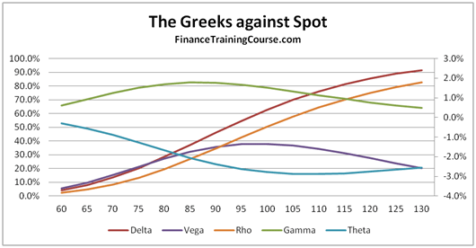
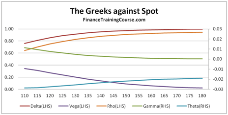
Figure 1 The Five Greeks. Plotted against changing spots

The image above presents a plot of the five factors for an At The Money (ATM) European call option.

Delta (Spot Price)- Measures the change in the value of the option price, based on a change in price of the underlying. Delta is the dark red line in the image above.

Vega (Volatility) – Measures the change in the value of the option price, based on a change in volatility of the underlying. Vega is the dark indigo line in the image above.

Rho (Interest Rates) – Measures the change in the value of the option price based on a change in interest rates.

Theta (Time to expiry) – Measures the change in the value of the option price based on a change in the time to expiry or maturity.

The first four sensitivities measure a change in the value of the option price based on a change in one of the determinants of option prices – spot price, volatility, interest rates and time to maturity. The fifth and final sensitivity is a little different. It doesn’t measure a change in option price, but measures a change in one of the sensitivities, based on a change in the price of the underlying.

Gamma – Measures a chance in the value of Delta, based on a change in the price of the underlying. If you are familiar with fixed income analytics, think of Gamma as Delta’s convexity.

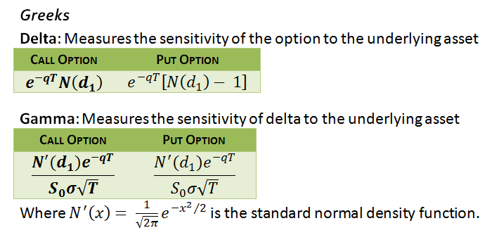
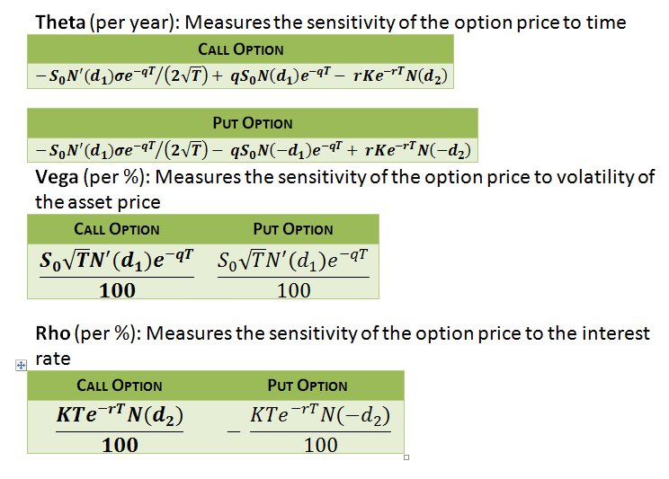
As promised above, we won’t hit you with any equations. However a quick notation summary is still required to appreciate the shape of the curves you are about to see.

Delta, Vega, Theta and Rho are all first order changes, while Gamma is second order change. If you take a quick look at the plot of the five factors presented above, you will see that the shape of the curves are similar for Delta and Rho (the slanting S) and similar for Gamma, Vega and Theta (the hill or inverted U). We will revisit the shape debate later on in our discussion.

Sales and Trading Interview Guide: Let’s talk about Delta

Delta has a handful of interpretations. Some common, some exotic.

The common interpretation is the one we have just covered above. Delta tracks option price sensitivity to changes in the price of the underlying. The second interpretation is as a conditional probability of terminal value (St) being greater than the Strike (X) given that St > X for a call option.

The third and the most relevant definition to our discussion comes from the option replicating and hedging portfolio example from the Black Scholes world.

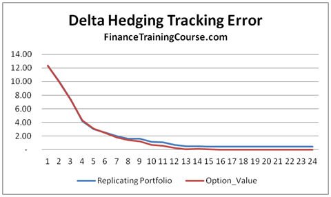
Figure 3 Delta Hedging. Replicating portfolio for call option using option Delta

As a seller of a call option if you would like to hedge your exposure (short call option) so that when (or if) the call option is actually exercised your loss is ideally completely offset by the change in value of your replicating portfolio.

This replicating portfolio is defined as a combination of two positions. A long position in the underlying given by Delta x S, less a borrowed amount.

Figure 4 – The Delta Hedge Relationship

For a European call option Delta is defined as

If we adjust Delta and with it the borrowing amount at suitably discrete time intervals we will find that our replicating portfolio will actually shadow or match the value of the option position. When the option is finally exercised (or not exercised) the two positions will offset each other.

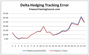
Figure 5 Delta Hedging. Replicating portfolio performance for hedging a short call option exposure

The two replications snap shots shown above show how closely the two portfolios move with changes in the underlying price over a one year time interval with fortnightly rebalancing (24 time steps). The tracking error will reduce if the rebalancing frequency is increased but it will also increase the cost of running the replicating portfolio.

Now that we have gotten the basic introduction out of the way, let’s spend some time on dissecting Delta by evaluating how this measure of option price sensitivity changes as you change:

a) Spot,

b) Strike,

c) Time to expiry and

d) Volatility.

Where relevant and important, we will add more context by also looking at how Delta’s behavior changes if the option is in, at, near or out of money.

Sales and Trading Interview Guide: Dissecting Delta – Against Spot

So how does Delta behave across a range of spot prices.

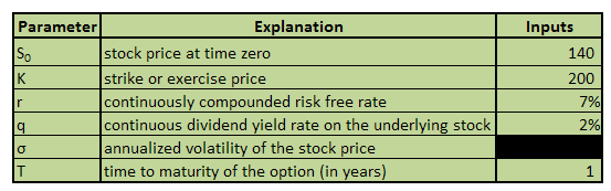
If we assume that we have purchased or sold a call option on a non-dividend paying stock with a strike price of US$100. The underlying is currently trading at a spot price of US$100. The time to expiry or maturity is one year.

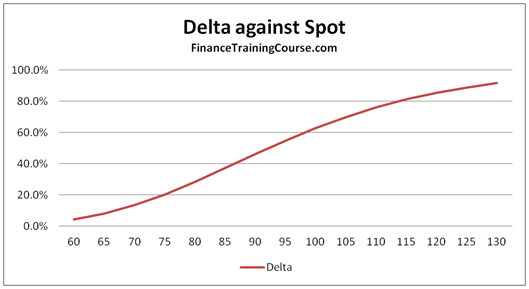
Figure 6 Delta plotted against changing spot prices

The graph above shows the change in the value of Delta as spot prices move higher or lower from the original US$100.

In this specific instance while we have moved spot prices we have held maturity constant. As a result while spot prices for the underlying change from 60 to 130, the option’s delta doesn’t touch zero or 1, since there is a chance that it may still switch direction and go the other way.

How does the behavior of Delta change if you move across At money options to options that are deep out of money or deep in the money? Think about this for a second before you move forward. Would you expect to see a different curve? Or a different shape? How different?

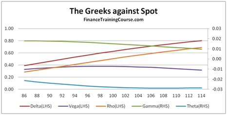
Let’s start with at, in and near money options.

For at money or near money options the shape remains the same. For options that are deep in the money, it becomes asymptotic before finally touching 1. From our hedging definition above, this means that the seller of the option should now own the exact numbers of shares of the underlying committed to the call option (Delta = 1) since the option will most certainly expire in the money. From a probability definition perspective, for a call option a conditional probability of 1 indicates that the option is certain to expire in the money.

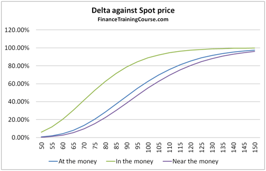
Figure 7 Delta against Spot. At, In and near money options

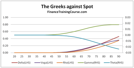
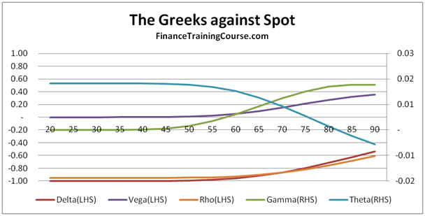
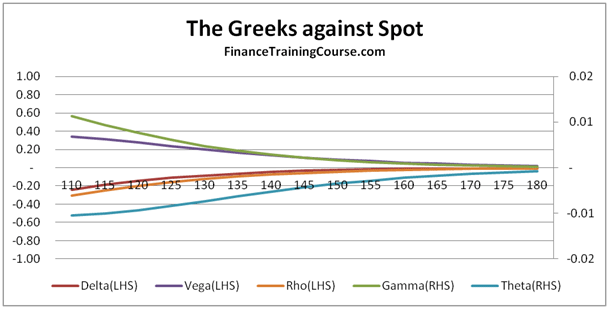
But what about deep out of money options? What happens to Delta or for that matter to all the other Greeks discussed earlier when it comes to deep out of money options.

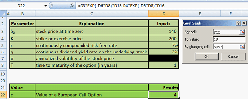
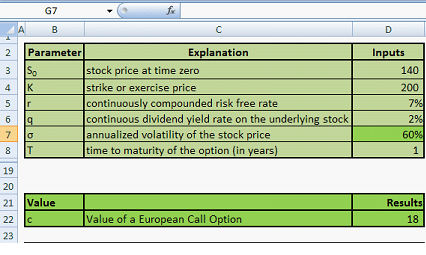
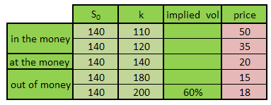
We answer this question by plotting the Greeks for a European call option written with strike price of US$200, while the current spot price is only at US$100. In the price ranging between US$60 and US$130, the value of Delta touches zero and then slowly rises to about 8% as the underlying spot price reaches US$130.

The overall shape remains the same, all we are doing now is just looking at a different pane of the option sensitivity window. Slide a little further or put the two images (figure 7 and figure 8) side by side and you should be able to see the complete picture.

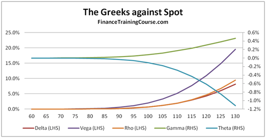
Figure 8 The Greeks against Spot. Deep out of money options

Figure 9 The Greeks against spot. AT, In and near money options

The next natural question deals with the valid range of values that Delta is expected to take. For a call option the range is between 0 and 1, as we have seen demonstrated above. Zero for deep out of money options, one for deep in money options. In between for all other shades.

For put options, Delta ranges between 0 and -1. Deep in money put options touch a Delta of -1, deep out of money put options reach a Delta of zero. The negative sign corresponds to a short position. To hedge a put, unlike a call, we short the underlying and invest the proceeds, rather than buy the underlying by borrowing the difference.

Sales and Trading Interview Guide: Dissecting Delta & Gamma – Against Strike

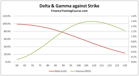
Figure 10 Delta & Gamma against changing strike price.

The next graph plots Delta and Gamma against changing strike price. We use a plot of both Delta and Gamma to reinforce the relationship between the two variables. Once again before you proceed further think about why do you see the two curves behave the way they do?

As the strike price moves to the right, the option gets deeper and deeper out of money. As it gets deeper in the deep out territory, the probability of its exercise and the amount required to hedge the exposure fall. Hence the steady decline in Delta as the strike price moves beyond the current spot price.

As the rate of change of Delta increases, we see Gamma rise by a proportionate amount. Gamma will only flatten out once the rate of change of Delta flattens out in the image above.

Sales and Trading Interview Guide: Dissecting Delta & Gamma – Against Time

The next three plots show how Delta and Gamma change as we vary time to expiry from a day to one year.

In the three snapshots that follow below, time moves from right to left (more to less). Once again we use both Delta and Gamma to reinforce the relationship between the two factors.

The only other variation from the options above is that we are now looking at three different options. An at money Call (Spot = 100, Strike = 100), an in money call (Spot = 110, Strike = 100) and a deep out of money call (Spot = 100, Strike = 200).

Notice how delta declines with time for an at money call, but rises to 1 for an in money call. Beyond a certain cut off point, it also rises for a deep out of money call but not as much as our first two pairs.

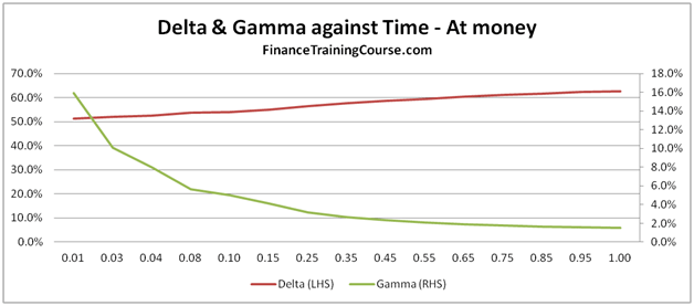
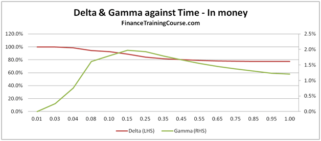
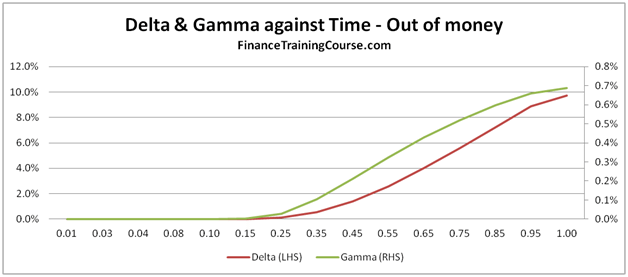
Figure 11 Delta & Gamm against Time for in, at and out of money options

Sales and Trading Interview Guide: Dissecting Delta & Gamma – Against Volatility

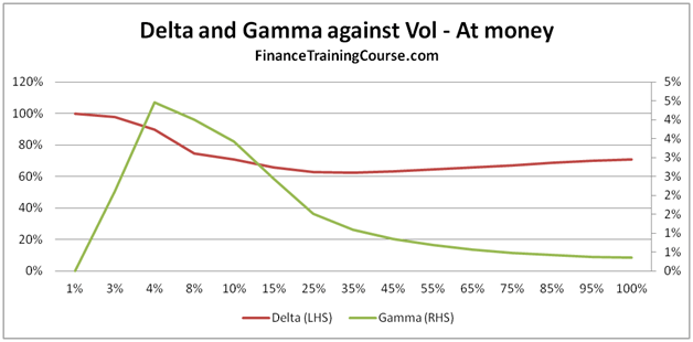
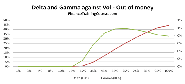
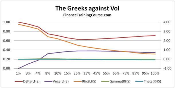
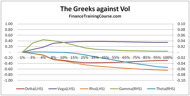
Figure 12 Delta, Gamma against Volatility. For at and out of money options.

For our last act, we plot Delta and Gamma against volatility and see a result which some students find counter intuitive.

For in, near or at money option, Delta actually falls with rising volatility. For most students this is a surprising result. Once would expect that with rising volatility, the value of the option should go up (correct) because the range of values reachable by the underlying is higher (also correct) hence leading to a higher probability of exercise (incorrect).

For deep out of money options, Delta rises with rising volatility. Gamma keeps pace initially but then runs out of steam as the rate of increase in Delta begins to flatten out.

To appreciate this behavior you actually have to move away from the Greeks and look at exercise probabilities.

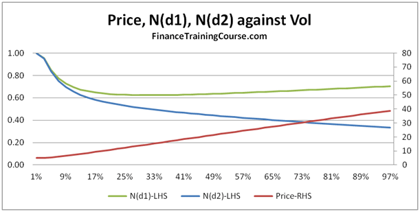
Understanding the relationship between volatility, probability of exercise and price.

Our next three plots, show how the conditional probability of exercise N(d1), the unconditional probability of St > X, N(d1) and price behave and change for in, at and out of money European call options.

In the images beneath, Price is measured using the right hand scale, while the two probabilities are measured using the left hand scale.

For at, in and near money options, the two probabilities actually decline as volatility rise. Sounds counter intuitive when you consider that while the two probabilities are declining, the price of the option is actually rising.

Here is a hint, look up and think about volatility drag. For a deep out of money option the trend is reversed. Once again ask yourself why?

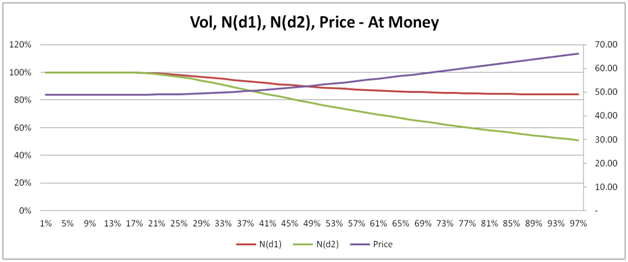
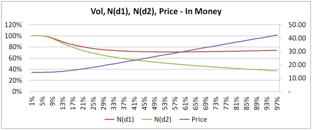
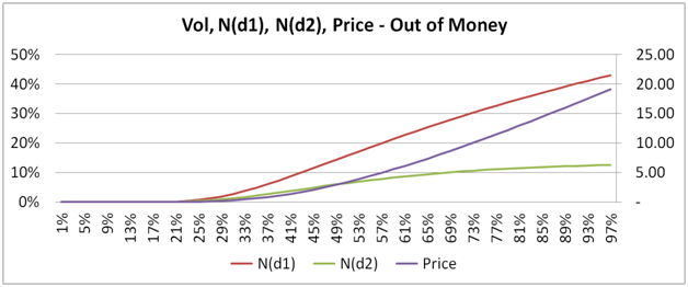
Figure 13 Vol, N(d1), N(d2) and Price for in, at, and deep out of money call options

Understanding Greeks: Option Delta and Gamma Review. Conclusion

If you are interested in a career on the floor or on a derivatives trading desk, you need to get very comfortable with the above graphs and behavior of Greeks across them. To the point of the lessons discussed becoming second nature – like riding a bike, breathing or drinking coffee. To remove the shock and awe caused by the partial differential equations behind the Greeks, we completely eliminated them from this post. In real life and when modeling them in excel you will have to get re-acquainted. Drop us a line with your questions or other dimensions that you would like us to address and if we can, we will do a few more posts on this topic.

Enjoy.

No related posts.