A brew of Volatilities – Implied volatilities, a simplified illustration
This post needs an understanding of the Black Scholes option pricing model (Black Scholes pricing reference). We will discuss at a very simplistic level:
- Implied volatility
- Volatility smile
Implied Volatility – Background
In the Black Scholes Merton option pricing framework all parameters are generally known and reasonably stable other than expected future realized volatility. In the academic world we are happy with using historical or empirical volatility as a proxy for future realized volatility but that doesn’t work on a trading desk.
Implied volatility is one way of calibrating option pricing models based on market prices and using market expectations of future volatility rather than historical volatility.
The process for finding implied volatility is the reverse of pricing an option; take the market price of an option, then derive the implied volatility from that price. In other words, now that we know the output, arrive at input volatility using this market price. Hence the name implied volatility.
For our discussion we will consider in-the-money, out-of-money and at-the money options.
Implied volatility – a simple case – calculating implied volatility using excel
We start with out of money call options with one year to expiry. Assume we have the following inputs:
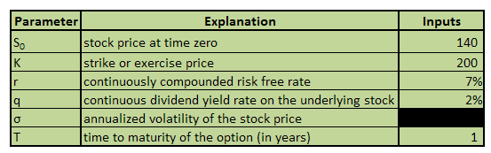
Figure 1 – Implied volatility using excel – Inputs
Note that r, q and T will remain the same for all the cases. We are interested in just changing the stock price at time zero S0 and the strike price k and then use the market price to arrive at the implied volatility.
The volatility box is shaded black because we are still in the dark as to its value.
For this set of inputs, the market price of call option is $18. Now we utilize the excel function of ‘Goal seek’. What is the volatility that will be generate a Black Scholes price of $18? The image below shows the Goal seek setup
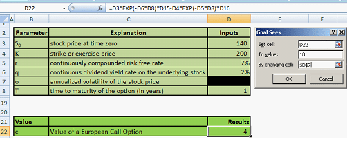
Figure 2 – Using Goal Seek to calculate implied volatility
Go to Data tab in Excel, then ‘What-if’ Analysis and then select Goal Seek. Currently value of the call is $4 for a given volatility. However we want to set this equal to $18 by changing cell D7 which is volatility. Press ok.
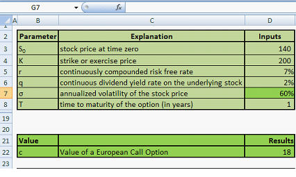
Figure 3 – Implied volatility using excel – result of the Goal Seek
The Goal seek result is an implied volatility of 60%.
Using the same goal seek function and the approach specified above we attempt to fill the following table:
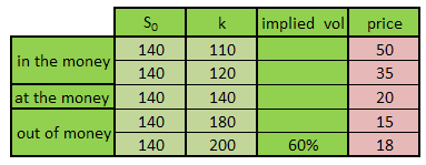
Figure 4 – Implied volatility – unfilled table
Note that the price is shaded pink and already filled in. This means that the price is not calculated but taken from traders for a call option with respective strike and spot price at time zero.
Using the goal seek function 4 times, the table is filled and shown below:
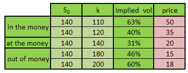
Figure 5 –Implied volatilities – filled table
Introducing the Volatility smile
Now plot the implied volatility by keeping strike price k as the x-axis.
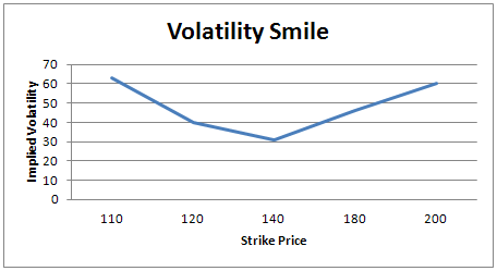
Figure 6 –Volatility smile
See this curve which looks like a smile? This is the volatility smile. How do we interpret this?
Volatility smile is the observation that an at-the-money options exhibits lower implied volatility than deep out-of-the-money and deep in-the-money options.
Volatility smile is the hole in the constant volatility assumption of Black Scholes. It came to prominence after the 1987 stock market crash.
The journey to modeling volatility smile
The first work was of Hull and White that took ‘stochastic volatility’ as the solution for the smile problem. However, this required a second parameter to be calculated which could not be observed directly, i. e, the market price of volatility risk. The model was also not arbitrage free.
The same challenge applies to jump-diffusion models. This family of models also introduced other parameter(s) that were not observable directly.
Derman and Kani utilized the binomial method. This does not introduce another unobservable parameter and the emphasis in on fitting the data. Another factor lambda is introduced which is calculated as per market prices. Using Arrow-Debreu prices with a binomial tree leads to implied tree .Implied trees result in market consistent prices for plain vanilla as well as exotic options. The Derman Kani model for implied volatility is also arbitrage-free.
However Paul Wilmott criticizes the binomial method calling it a ‘dinosaur’ that takes too much time to yield results.
Other quants look at volatility smile problem in a different manner. The existence of volatility smiles contradicts the normality assumption of Black Scholes as well. The main culprits are skewness and kurtosis. This means that the distribution is more ‘peaked’ at the mean and has thicker tails. Adjustment terms in the Black Scholes are added to account for kurtosis and skewness.
Implied volatilities: Models on models
The main short coming of all the models is that although these theoretical models are consistent with the smile, the statistics and facts show that the smile is about twice as large as predicted by these models; something else is going on.
Ongoing research shows that trading costs are largely to blame for this. Picturing an individual security’s returns with the relative market context and the uncertainty associated with it also causes concerns relating to the shape of the implied volatility.
Implied Volatilities. Conclusion
There is still much research needed before we can reach a solid conclusion as to how to precisely model volatility smile. The common thread researches share however is that there are monetary aspects like trading costs responsible driven by market participant behavior.
Sources
http://202.112.126.97/jpkc/jrysgj/files/18.Why%20do%20we%20smile%20On%20the%20determinants%20of%20the%20implied%20volatility%20function.pdf
http://www.ederman.com/new/docs/gs-volatility_smile.pdf
Related posts:
- Financial Risk Management Workshop – Value at Risk, Volatility and Trailing correlations – Day One
- Advance Risk Management Models – Workshop & Training reference page
- Forwards and Swaps: Interest Rates Models: Bootstrapping the Zero curve and Implied Forward curve