Rebalancing frequency, Implied Volatility & Rho. Dynamic Delta Hedging Applications.

Now that we have a Delta Hedging Model for Calls and Puts let’s try and use it to answer the following questions:

a) What is the impact of rebalancing frequency on hedging profitability?

b) What is the impact of a rise in volatility on profitability? How does implied volatility help in interpreting this change?

c) What is the impact of changes in risk free rates on profitability?

d) How does the interaction of time to expiry and volatility changes profitability?

These are all questions that should occur naturally to you as you spend more time with the Delta Hedging model. They are also essential to building a deeper understanding of the concept of implied volatility, Rho & Theta.

Dynamic Delta Hedging Questions: Assumptions & Securities

Let’s take a look at these questions one by one. We will begin work with a call option assuming the following valuation parameters:
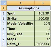
Figure 1 Dynamic Delta Hedging – P&L review assumptions

The theoretical value of the call option is 3.01 based on the above assumptions. The resulting Cash Accounting P&L for a single run of the Dynamic Delta Hedging model is as under:
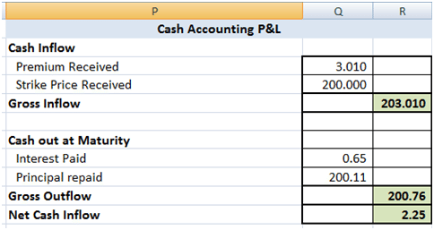
Figure 2 Dynamic Delta Hedging – P&L Review – Base case

Rebalancing frequency & efficiency of the hedge. Implications for profitability?

A good hedge is one where the cost of the hedge is close to the theoretical value of the option. In our cash accounting P&L we have included the theoretical premium received which is used in determining the initial amount to be borrowed. Hence for a hedge to be considered good or efficient the Net P&L should be close to this premium amount.

To see if increasing the frequency led to better results, we increase the time steps used from 12 steps to 365 steps. The graph below plots the Net P&L to Theoretical Value across 100 simulated runs. A value close to 100% means that it is a close match to the premium whereas a value farther away for 100% indicates a poor match.
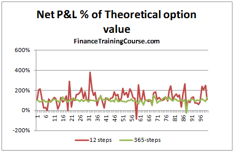
Figure 3 Dynamic Delta Hedging – P&L Simulation – Rebalancing frequency

We can clearly see that there is much greater variation when the rebalancing is done on a monthly basis than when it is carried out on a daily basis.

The graph below gives a similar picture. In this case however, the premium is not considered when determining the amount to be borrowed at option inception, i.e. the hedge is fully funded through borrowing. A value of -100% indicates that the Net P&L i.e. the cost of the hedge, in this case exactly matches the theoretical value of the call option.
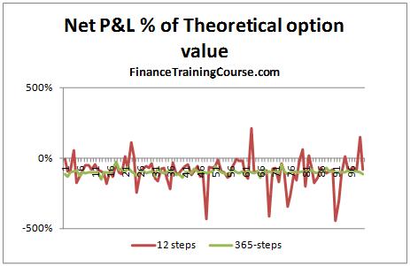
Figure 4 Dynamic Delta Hedging – P&L Simulation – Hedge Effectiveness

But that is the risk manager’s point of view. What about a trader’s point of view?

From a trading point of view there are two lessons here. First the large variation in P&L linked to jump’s in the underlying price is the un-hedged Gamma at work (Is that true? Think about it). Second would you prefer to limit the cost of hedging the option to the amount you have charged your customer or less? If you are in the business of earning a living from writing options, the premium you charge on the options you sell should always be higher than your cost; your cost of effectively hedging the option.

Now back to the Gamma question. Gamma is your second order error term. Conceptually it’s similar to convexity and linked to changes in not just the underlying price but also volatility. Is your true P&L (the premium received less the actual cost of hedging) is the summation of the hedge error?

Volatility and profitability. The question of implied volatility

With volatility there are multiple questions. How does profitability change when the general environment moves from low volatility to high volatility? How does profitability change when you have already written an option and volatility moves for or against you?

Let’s start from the first question. Using the 12-step model we calculate the impact on Net P&L. In our base case we have assumed a volatility of 20%. Let us now assume that the volatility increases to 40%. What is the impact on hedge efficiency for options written in the two different environment?
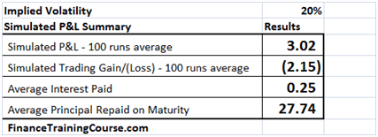
Figure 5 Volatility & Profitability – Low volatility world
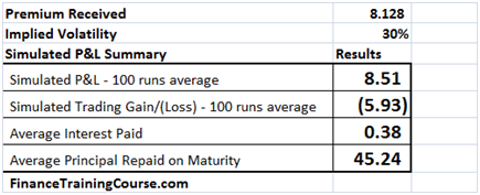
Figure 6 Volatility & Profitability – High Volatility world

So premiums are clearly higher and so is profitability in absolute terms. But is that true in the relative world? Let’s take a quick look by plotting the Net P&L to Theoretical Value across 100 simulated runs. In relative terms (as a % of premiums) there is not much difference. Why is that? Is this a result you expected?
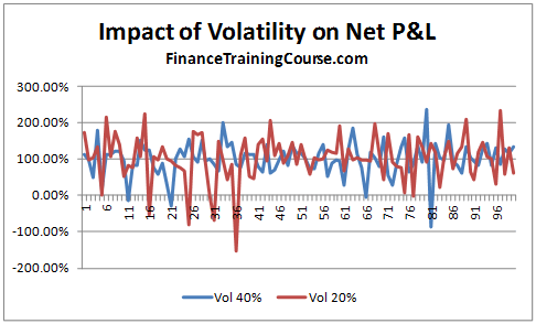
Figure 7 Dynamic Delta Hedging – P&L Simulation – Volatility Impact

To answer these questions you have to revisit implied volatility. Let’s use the same scenario as above but with a minor change. We wrote options and received premiums assuming an implied volatility of 30%. The actual realized volatility over the life of the option was 20%. How did that change our resulting simulated P&L.
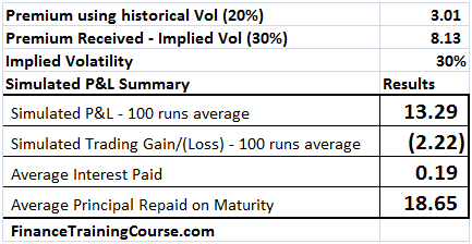
Figure 8 Implied volatility at work – Hedge Profitability

You can now see a clear difference in absolute as well as relative terms in net P&L. And the difference arises on account of the spread between the premium charged ($8.13) versus the premium needed ($3.01).

(To run this exercise using the Delta Hedge Sheet, simply calculate the value of the premium at the implied volatility level you want to charge and replace the original premium in the simulation with this value).

Risk free rates & profitability. The question of Rho.

We present the results of three P&L simulations runs in the tables below. The first assumes a risk free interest rate of 1%, the 2nd uses 2% and the third uses a risk free interest rate estimate of 5%.

The first two are easy, rates go up, premiums goes up and a European Call option becomes more expensive. Why is that?
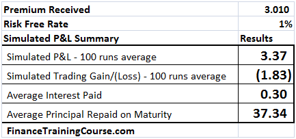
Figure 9 Dynamic Delta Hedging profitability – P&L at 1% interest rates

The reason is the average interest paid column. The premium goes up by 28 cents of which 21 cents is the increased cost of financing the borrowed position. Where does the other 7 cents comes from? (Need a hint – Other than the borrowing component who else benefits or uses r, the risk free rate?)

Figure 10 Dynamic Delta Hedging profitability – P&L at 2% interest rate

The second one is more difficult. In this instance as rates increase to 5% from the original 1%, the cost of borrowing balloons to $1.95 from the original $0.30 but the impact in option premium is only $1.244. How does this work? (Hint, think about what other driver/factor in the Black Scholes Analysis uses r?)
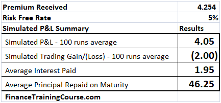
Figure 11 Dynamic Delta Hedging profitability – P&L at 5% interest rates

In addition to borrowing the difference between premium received and Delta hedge, the other usage of the risk free rate, r, is in estimating the future value of the underlying asset in the BSM (Black Scholes Model’s) risk neutral world. This implies that there are other components of Rho, in addition to the borrowing cost. That you need to examine and be comfortable with.

Understanding Greeks & Delta Hedging

Related posts:

  1. Understanding Delta Hedging for options using Monte Carlo Simulation
  2. Dynamic Delta Hedging – Calculating Cash PnL (Profit & Loss) for a Call Option writer
  3. Dynamic Delta Hedging – Extending the Monte Carlo simulation model to Put contracts

Practice Exam Test Question – Pricing and MTM of Interest Rate Swaps (IRS)

And now for the last and final part of our Practice Exam Test Question series on Pricing Interest Rate Swaps (IRS). In our first post we walked through the process of building a annualized forward curve and then extending it to semiannual rates.

In this post we will take the forward curve generated in the previous post and use it answer our Interest Rate Swaps (swap rate) and mark to market (valuation) questions.

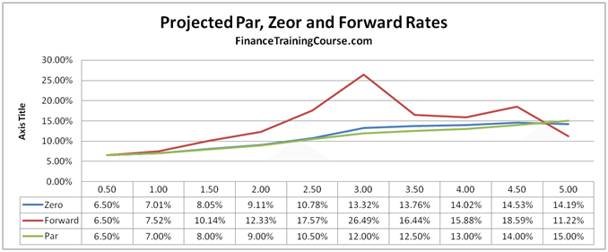
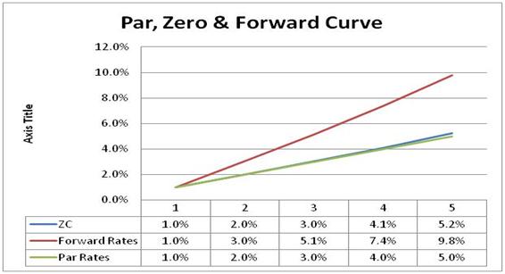
Here is the projected zero and forward rates curve from our previous post, posted here for convenience. Before you proceed further please take a quick look at the interest rate swap pricing free study guide to review our approach and methodology.

Mark to Market and Valuing an Interest Rate Swap – Practice Test Question and Partial solution

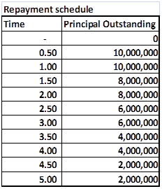
A client has recently entered into a 4.5 year floating rate loan for US$ 400,000,000? The loan will be effective six months from now and will use the following repayment schedule.

Figure 1 Practice Exam Question – Notional Principal for pricing Interest Rate Swaps

The client has asked for a quote for the an effective interest rate risk hedge that would offset the risk of rising interest rates.


a)
What would be the swap rate at cost or breakeven basis for this structure?


b) Would the client be paying fixed or receiving fixed


c) What would be the swap rate if the loan starts at time 2.5 with 10,000,000 and ends at time 3 with an outstanding principal of 10 million.


Here is the output from our solution Excel Sheet. The approach is as per interest rate swap pricing free study guide. The projected forward rates are as per the results above and were driven in the projected forward rates using bootstrapping post. As you can see that the trick here was recognizing that we didn’t have a normal interest rate swap but a forward starting amortizing swap and then adjust the pricing approach accordingly.


a) The exact breakeven swap rate is 13.718% and the breakeven value of each leg (fixed and floating) is 3.001609
million.

b) Since the client is hedging a floating rate loan with this swap he will be paying a fixed rate and receiving the floating rate or simply paying fixed.


Figure 2 The practice test question solution – the interest rate swap pricing, MTM and valuation grid

c) This question is asking you to price a one step FRA or a Forward Rate Agreement. To solve it you should pick the row corresponding to tenor 2.5 and solve for a fixed rate that allows the present value of fixed and floating payments to completely offset each other. This fixed rate is 17.5732%. If you understood the question intuitively you should be able to answer it without resorting to the below solution by simply looking at the applicable forward rate and using that as the breakeven rate.


Figure 3 The practice test question – the FRA pricing, MTM and valuation grid

Common Interest Rate Swap pricing and valuation mistakes made by students in this question

  • Not making the forward pricing adjustment for the forward starting interest rate swap
  • Not using the correct notional amount. A number of students used a flat value of 400 million rather than the amortization schedule shared with the question above. Use the correct amortization schedule
  • Not adjusting for the day count in the fixed as well as floating cash flows. Students often use the full rate when calculating semiannual payment, where as they should be using 180/360 or 182/365 * the relevant interest to account for the fact that the payment is a semiannual interest payment.
  • Not using the correct applicable floating (forward rate)


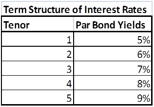
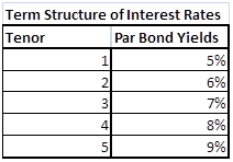
d) Six month later the interest rates term structure has changed as shown below. Taking the original Swap structure and assuming that the Swap was purchased at the original breakeven Swap rate, what is the MTM (Mark to Market value of the Swap).


Figure 4 Practice Exam question – Revised Interest Rate Yield Curve

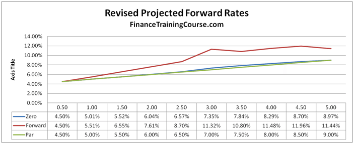
This question requires a simple re-application of the above process one more time. Here are the revised projected forward rates

Figure 5 Revised projected forward rates

The trick now is to remember that we have all moved 6 months forward in time and the IRS is effective now. Based on this assumption this is how the revised grid looks like. The IRS has a negative MTM because we had expected rates to go up and they have actually come down.

Figure 6 Pricing, MTM, Valuing the IRS under the new term structure and yield curve

Once again the biggest mistake students made here was not moving forward in time and pricing the IRS on an as is basis. The second biggest mistake was not using the updated curve and the old Swap Rate calculated from the earlier part of the question.

Related posts:

  1. Pricing Interest Rate Swaps – Derivative pricing final exam question for practice exams & test prep
  2. Practice Test Exam Question and Solution – Bootstrapping Zero and Forward Curves Case Study
  3. Online Finance Course – Pricing Interest Rate Swaps – Process

Pricing Interest Rate Swaps – Final Exam question for test prep

I teach the Derivative Pricing and Risk Management courses to EMBA and MBA students in Dubai and Singapore. In a recent exam one question caused a lot of heart ache and pain in exam takers. While most student understood the gist of the question, they still made a number of small mistakes that cost them valuable points in the final score.

If you have an interest rate swap pricing exam or test coming up, here is the sample question that you can use as a practice exam or practice test question. If you detailed hands on model building interviews for your Sales & Trading, FICC or Risk Management desks, the question has a few twists that can reveal how detail oriented and hands on your candidate is.

For best results, first try the exam and the practice and test question and then work through the solution (to be presented in the next post). Do the question under exam conditions and try and attempt the practice question in one sitting.

Best of luck for your exam.

Pricing Interest Rate Swaps – Practice Exam – Test prep question

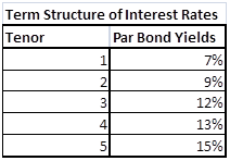
You are given the following term structure of interest rates for US$ using Yield to Maturity (YTM) of Par bonds that pay interest on a semi-annual basis

Figure 1 Test Prep – Practice Exam – The Interest Rates Yield Curve

Using these Par Bond Yields please answer the following questions:

7. Plot the following graph shown in Figure 1 using the above term structure and assuming that that coupon/interest is paid on a Semi Annual basis. This implies that you would need to build a 10 x 10 grid at semi-annual intervals for 5 years. Your graphical plot will show projected rates at 10 points at 10 half years. (15 Points)

Figure 2 Practice Exam – Sample Par, Zero & Forward curve plot


Please see the next page for question number 8

8. A client has recently entered into a 4.5 year floating rate loan for US$ 400,000,000? The loan will be effective six months from now and will use the following repayment schedule. (35 points)

Figure 3 Practice Exam Question – Notional Principal for pricing Interest Rate Swaps


The client has asked for a quote for the an effective interest rate risk hedge that would offset the risk of rising interest rates.


a)
What would be the swap rate at cost or breakeven basis for this structure?


b) Would the client be paying fixed or receiving fixed


c) What would be the swap rate if the loan starts at time 2.5 with 10,000,000 and ends at time 3 with an outstanding principal of 10 million.


d) Six month later the interest rates term structure has changed as shown below. Taking the original Swap structure and assuming that the Swap was purchased at the original breakeven Swap rate, what is the MTM (Mark to Market value of the Swap).


Figure 4 Practice Exam question – Revised Interest Rate Yield Curve

Related posts:

  1. Derivative Pricing – Interest Rate Swaps and Futures – Calculation reference
  2. Online Finance Course – Pricing Interest Rate Swaps – What is a Swap?
  3. Online Finance – Pricing Interest Rate Swaps – The valuation course

A brew of Volatilities – Implied volatilities, a simplified illustration

This post needs an understanding of the Black Scholes option pricing model (Black Scholes pricing reference). We will discuss at a very simplistic level:

  • Implied volatility
  • Volatility smile

Implied Volatility – Background

In the Black Scholes Merton option pricing framework all parameters are generally known and reasonably stable other than expected future realized volatility. In the academic world we are happy with using historical or empirical volatility as a proxy for future realized volatility but that doesn’t work on a trading desk.

Implied volatility is one way of calibrating option pricing models based on market prices and using market expectations of future volatility rather than historical volatility.

The process for finding implied volatility is the reverse of pricing an option; take the market price of an option, then derive the implied volatility from that price. In other words, now that we know the output, arrive at input volatility using this market price. Hence the name implied volatility.

For our discussion we will consider in-the-money, out-of-money and at-the money options.

Implied volatility – a simple case – calculating implied volatility using excel

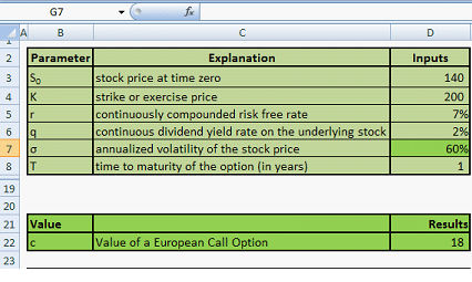
We start with out of money call options with one year to expiry. Assume we have the following inputs:

Figure 1 – Implied volatility using excel – Inputs

Note that r, q and T will remain the same for all the cases. We are interested in just changing the stock price at time zero S0 and the strike price k and then use the market price to arrive at the implied volatility.

The volatility box is shaded black because we are still in the dark as to its value.

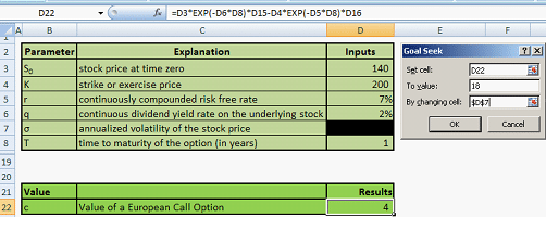
For this set of inputs, the market price of call option is $18. Now we utilize the excel function of ‘Goal seek’. What is the volatility that will be generate a Black Scholes price of $18? The image below shows the Goal seek setup


Figure 2 – Using Goal Seek to calculate implied volatility

Go to Data tab in Excel, then ‘What-if’ Analysis and then select Goal Seek. Currently value of the call is $4 for a given volatility. However we want to set this equal to $18 by changing cell D7 which is volatility. Press ok.

Figure 3 – Implied volatility using excel – result of the Goal Seek

The Goal seek result is an implied volatility of 60%.

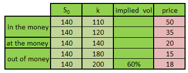
Using the same goal seek function and the approach specified above we attempt to fill the following table:

Figure 4 – Implied volatility – unfilled table

Note that the price is shaded pink and already filled in. This means that the price is not calculated but taken from traders for a call option with respective strike and spot price at time zero.

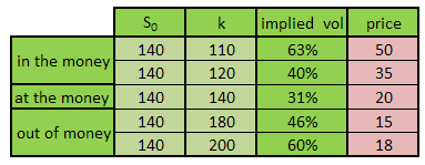
Using the goal seek function 4 times, the table is filled and shown below:

Figure 5 –Implied volatilities – filled table

Introducing the Volatility smile

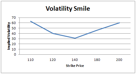
Now plot the implied volatility by keeping strike price k as the x-axis.

Figure 6 –Volatility smile

See this curve which looks like a smile? This is the volatility smile. How do we interpret this?

Volatility smile is the observation that an at-the-money options exhibits lower implied volatility than deep out-of-the-money and deep in-the-money options.

Volatility smile is the hole in the constant volatility assumption of Black Scholes. It came to prominence after the 1987 stock market crash.

The journey to modeling volatility smile

The first work was of Hull and White that took ‘stochastic volatility’ as the solution for the smile problem. However, this required a second parameter to be calculated which could not be observed directly, i. e, the market price of volatility risk. The model was also not arbitrage free.

The same challenge applies to jump-diffusion models. This family of models also introduced other parameter(s) that were not observable directly.

Derman and Kani utilized the binomial method. This does not introduce another unobservable parameter and the emphasis in on fitting the data. Another factor lambda is introduced which is calculated as per market prices. Using Arrow-Debreu prices with a binomial tree leads to implied tree .Implied trees result in market consistent prices for plain vanilla as well as exotic options. The Derman Kani model for implied volatility is also arbitrage-free.

However Paul Wilmott criticizes the binomial method calling it a ‘dinosaur’ that takes too much time to yield results.

Other quants look at volatility smile problem in a different manner. The existence of volatility smiles contradicts the normality assumption of Black Scholes as well. The main culprits are skewness and kurtosis. This means that the distribution is more ‘peaked’ at the mean and has thicker tails. Adjustment terms in the Black Scholes are added to account for kurtosis and skewness.

Implied volatilities: Models on models

The main short coming of all the models is that although these theoretical models are consistent with the smile, the statistics and facts show that the smile is about twice as large as predicted by these models; something else is going on.

Ongoing research shows that trading costs are largely to blame for this. Picturing an individual security’s returns with the relative market context and the uncertainty associated with it also causes concerns relating to the shape of the implied volatility.

Implied Volatilities. Conclusion

There is still much research needed before we can reach a solid conclusion as to how to precisely model volatility smile. The common thread researches share however is that there are monetary aspects like trading costs responsible driven by market participant behavior.

Sources

http://202.112.126.97/jpkc/jrysgj/files/18.Why%20do%20we%20smile%20On%20the%20determinants%20of%20the%20implied%20volatility%20function.pdf

http://www.ederman.com/new/docs/gs-volatility_smile.pdf

Related posts:

  1. Financial Risk Management Workshop – Value at Risk, Volatility and Trailing correlations – Day One
  2. Advance Risk Management Models – Workshop & Training reference page
  3. Forwards and Swaps: Interest Rates Models: Bootstrapping the Zero curve and Implied Forward curve