Dynamic Delta Hedging – Calculating Cash PnL (P&L) for a European Call Option

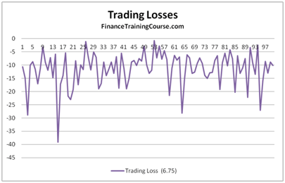
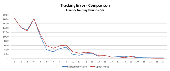
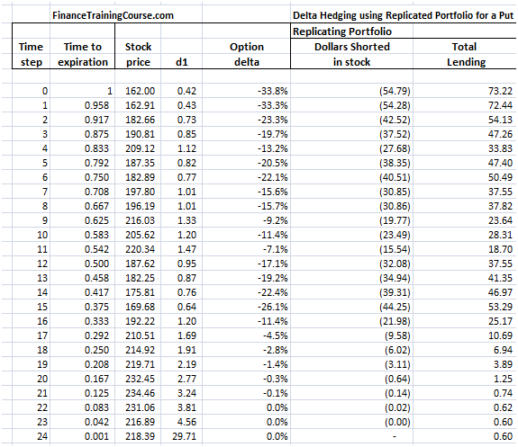
Figure 1 Delta Hedge P&L – Trading losses on account of rebalancing

We extend the original Dynamic Delta Hedging Monte Carlo Simulation spread sheet in this note. The dynamic hedging spreadsheet for a European call option allowed us to do a step by step trace of a delta hedging simulation. In this sheet we will use the results from the simulation trace to calculate a cash accounting P&L for our hedging model assuming the role of a call option writer and then extend the original simulation to see the average PnL across 100 iterations.

The above calculation has a double count in it? Which directly impacts the final profitability figure? Can you see it? See the discussion below for an answer.

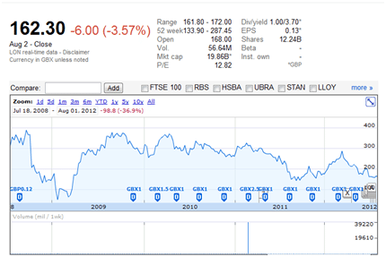
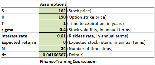
We are assuming that we have written a European call option on Barclays Bank where the current spot price is $162.3 and the strike price is US$200. Time to expiry is one year and Barclays Bank is unlikely to pay a dividend during the life of the option.

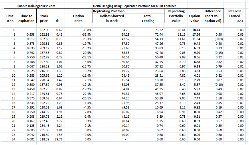
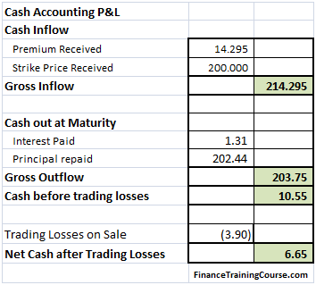
Figure 2 Delta Hedge P&L – Cash P&L for the writer for a call option that expires in the money

Understanding Delta Hedging Cash PnL Calculation – Required resources

Before you proceed further if you are still uncomfortable with option price sensitivities or delta hedging please use the following background and model review posts to make yourself comfortable with the underlying concepts.

  1. Understanding option Greeks reference resource for dummies
  2. Understanding Greeks – Analyzing Delta & Gamma
  3. Understanding Greeks – The Guide to delta hedging using Monte Carlo Simulation
  4. Understanding Greeks – The Delta Hedging Simulation extended for Put Options

Delta Hedging Cash PnL Calculations – Dissecting the PnL Model

Our model uses a simplified cash based approach to calculate PnL from our Delta Hedging model. Our objective is to calculate PnL at option expiry for the option writer. Primary contributors to the model include:

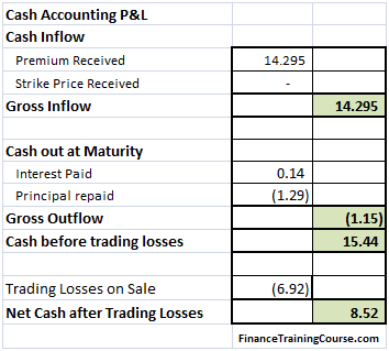
Figure 3 Delta Hedge – Cash P&L for the writer for an option that expires out of money

a) Cash in – receipts from the customer. Include premium received and the strike price if the option is exercised. If the option expires worthless we only receive the premium.

b) Cash out. As explained earlier to finance our hedge purchases we borrow money. We pay interest on this principal for the life of the hedge and return the principal at maturity.

c) Trading losses. As part of our strategy we purchase the underlying as prices rise and sell it when they fall. Be definition this strategy will generate trading losses irrespective of whether the option expires worthless or in the money. Because we re-balance on a frequent basis, trading losses also consume cash. However the question that often confuses audiences is one of double count. Should trading losses be included as a separate accounting item or are they already included in the Cash before trading losses calculation? Think about this before you proceed further. It will directly impact your analysis and result. Here is a hint – other than the cash treatment that we have used, is there any other possible use or source of cash in the analysis and the calculation above?

When we put the model in place our final output should look something like this:

Figure 4 Delta Hedge P&L Simulation results – Gross P&L, Net P&L, Trading Losses

You can clearly see that the biggest contributor to our cash PnL uncertainty is trading loss. Is this treatment correct?

We will take a more closer look at this contributor later in our note.

Extending the Delta Hedge Model for Cash PnL Calculation – Interest paid & principal borrowed for the Hedge

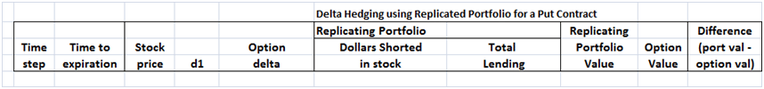
The first step is to add two new columns to our Delta hedge model. These are:

  1. Interest paid per period, and
  2. Incremental amount borrowed per period

Both elements have been calculated as part of the original sheet and all we need to do is simply extract the relevant piece and dump the results in two new columns at the end.

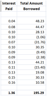
Figure 5 Delta Hedging PnL – Two new columns – Interest paid & Marginal borrowing

Incremental amount borrowed is included in the total borrowing figure we had calculated earlier in the Guide to delta hedging using Monte Carlo Simulation
post. It is simply the difference between the two deltas for the two time periods multiplied by the new price of the underlying stock.

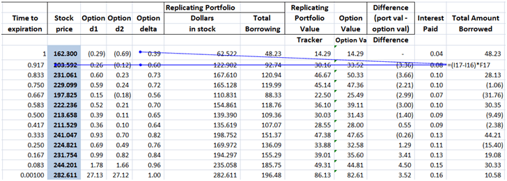
Figure 6 Delta Hedging PnL – Calculating Incremental borrowing

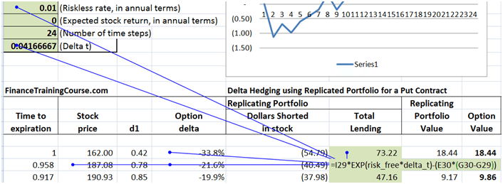
Interest paid per period is the interest accrued on the balance of the previous period. Which ends up as outstanding balance times the interest accrual factor (exp(risk_free_rate x Delta_T)) in the sheet.

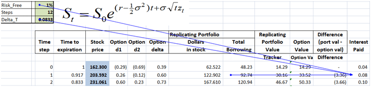
Figure 7 Delta hedging PnL – Calculating Interest paid on borrowed cash

Delta Hedging PnL – Calculating the trading loss on account of selling low

The basic hedging strategy is to buy when delta (or price) goes up and sell when delta (or price) goes down. Buy when prices rise, sell when they decline. The result is that as the underlying price see-saws, we end up buying high and selling low, rebalancing the portfolio in alignment with delta but also generating trading losses.

Our calculation of trading losses has three components.

a) First calculate the number of incremental units purchased or sold as part of the required rebalancing. (Unit purchased column)

b) Then calculate the difference in price between the two rebalancing periods. (Difference in price column)

c) Finally identify all trades where a sale was made and calculate the trading gain or loss. (Loss on Sale column)

For this specific simulation the trading loss is calculated as $2.5 based on the above approach.

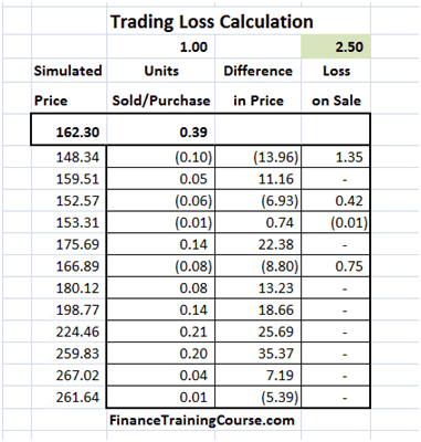
Figure 8 Delta Hedge simlation – trading loss calculation

Delta Hedge PnL Calculation – Putting it all together

Now that we have all of the required PnL components together we hook them up with our Excel Data Table. We use our Monte Carlo bag of tricks to store the results of 100 iterations. Stored components include Gross PnL (excluding trading losses), Net PnL (including trading losses), Interest Paid & Trading loss on rebalancing sales.

But there is a trick question here. Its the question that has always stumped students (and quite frequently me).  Here is the question. Is the correct P&L the Gross P&L or the Net P&L figure below? The net P&L subtracts the trading loss from the gross figure. Is that a double count? How would you explain and justify the answer? Is there a one word answer?

Think about these questions as you work through the numbers in the table below. We will do a post answering the double count question later.  In the interim period here is a hint. Try a fully funded (zero premium) strategy once you have built the sheet and see what happens to your P&L calculation.

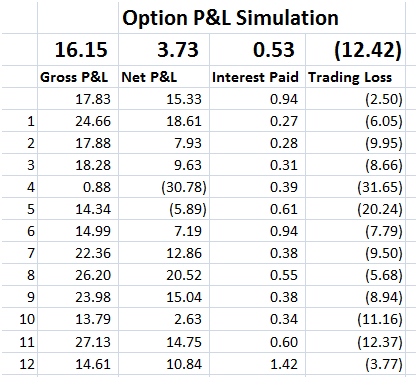
Figure 9 Delta Hedge PnL – Storing the results

(If this doesn’t make sense, take a quick look at our Monte Carlo Simulation refresher below.)

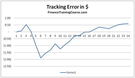
The final result is our Delta Hedge PnL graph for a European Call Option.

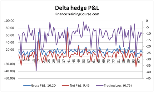
Figure 10 Dynamic Delta hedge PnL Calculation – PnL Graph

Delta hedging PnL – Next steps and Questions

Once you have the basic model figured out here are some interesting questions that follow:

a) How would you extend this model for PnL calculations for a European Put Option?

b) How would you incorporate the impact of implied volatility?

c) Of transaction costs? And non-risk free interest rates? Jumps and Dividends?

d) How would profitability (cash PnL) change if you shortened the time step and the rebalancing period? Or extended it?

e) What does the distribution of profits suggests about the risk inherent in the underlying business?

f) Is this the most effective way of hedging options?

g) What about the risk embedded in other Greeks? How is that managed and hedged? How does that impact PnL?


Understanding Greeks & Delta Hedging

Related posts:

  1. Dynamic Delta Hedging – Extending the Monte Carlo simulation model to Put contracts
  2. Understanding Delta Hedging for options using Monte Carlo Simulation
  3. The Sales and Trading Interview Guide Series – Understanding Greeks and Delta Hedging – Coming soon to an iPad near you…

Long billed Hoopoe or a crowned woodpecker?

A well rounded education in Finance includes an awareness of the environment around you.

This long billed bird has been prospecting in our office lawn for the last few months.  Armed with our Kite catching camera, we took a few sneak shots early this afternoon. The only question is that are we looking at  a long billed Hoopoe (probably) or a strange woodpecker (unlikely)?.  Lacking expertise in the accurate classification of this species, we thought it would be appropriate to simply post the question here and hope for the best.  Hope that some where in the audience there is a Quant who has been watching birds more closely than his Excel spreadsheets.

Long billed Hoopoe or a Woodpecker? You decide. (Need some help, check out the Woodpecker classification resource)


Side profile.

In action after a digging attempt is successful.


A full view of the crown on top from back


Getting ready to dig.

No related posts.

Dynamic Delta Hedging – Monte Carlo Simulation in Excel for hedging European put contracts

In our previous post on Dynamic Delta Hedging for European Call Options we built a simple simulation in model in Excel that simulated an underlying price series and a step by step trace of a Dynamic Delta Hedging simulation for a call option.

In this post we will modify and extend the model for European Put options. The basic approach remains the same but a simple modification is required to make the sheet work for European Put contracts.

Figure 1 Delta Hedging – Put Options – Monte Carlo Simulation

The end result would be a dynamic simulation graphical output showing the original option value and the replicating portfolio that is created to hedge it.

If you remember, our Dynamic Delta Hedging strategy for Call Options relied on going long (buying) Delta x S and financing this purchase by borrowing the difference between our purchase and the premium received for writing the option. This strategy defined the structure of our Monte Carlo Simulation spread sheet in Excel.

Figure 2 Delta Hedging – The baseline model and simulated values

Delta Hedge – Put Options – Tweaking the original Monte Carlo Simulation model

How would you change this model for hedging a European put contract?

In a call option the probability of exercise goes up as the underlying price goes up. For a put option the opposite is true. For a call option as the probability of exercise goes up, we buy portions of the underlying to hedge our exposure and manage our dollar cost average purchase price.

For a put option therefore we short more of the underlying as probability of exercise goes up ( the probability is N(d2) for a Call, N(-d2) for a Put) and vice versa when the probability goes down.

For a call because we are short cash we borrow it to finance our purchases. For a put option the short sale of the underlying generates cash and we invest the proceeds for the duration that we remain short.

Therefore the structure of our dynamic delta hedging sheet for a European put contract changes and becomes:

Figure 3 Dynamic Delta Hedging – Baseline model for European put options

The only difference are:

a) In the replicating portfolio: Where we are now short Delta x S and have lent the proceeds from the short sale

b) Option Delta calculation where we are using N(d1) – 1 rather than N(d1) as the option delta for a put option.

As per our earlier model we still need to simulate:

a) The underlying stock price

b) Option Delta for a put option linked to the underlying stock price

c) Replicating portfolio comprised of a short position in Delta x S (Spot price of stock) and a long position in Borrowing B.

d) Difference between the replicating portfolio and the option value to calculate tracking error.

Figure 4 Delta Hedging – Put Options – Tracking Error

If you are unfamiliar Monte Carlo Simulation please see the Monte Caro Simulation Training Guide below as well as our posts on Monte Carlo simulation before proceeding further.

We use Barclays Bank and assume that the bank will pay no dividends over the life of the option.

Delta Hedging Model using Monte Carlo Simulations – Assumptions

Figure 5 Dynamic Delta Hedging – Barclays bank price chart

Delta Hedge – Put Contract – Simulating the underlying using Monte Carlo Simulation

We will assume that the spot price is 162.3, the strike price 150, the daily volatility will range between 2.5% to 5%. Implied annualized volatility will be assumed to be 40%. Risk free rate of interest will be 1%, time to maturity will be one year. As discussed above, the stock will pay no dividends.

Figure 6 Delta Hedging – Key Assumptions

Using the above assumptions simulate a path of Barclays share price over the next one year. For each value of the underlying stock price we also calculate d1 using the standard Black Scholes European option pricing.

Figure 7 Delta Hedging – Put Option – Simulating the underlying

The actual stock price simulation with the original discrete formula and the Excel implementation is shown below and is the same as the approach used earlier for Delta Hedging. The only difference is that our Delta Hedging sheet worked with a 12 step forecast. For put options we are using a 24 step simulation.

Figure 8 Delta Hedging – Simulating the underlying

Armed with d1 we can now calculate option delta as well as the value of the replicating portfolio (Short Delta x S + Total lending).

Figure 9 Delta Hedging – Put Option – Completing the Picture

Delta Hedge – Put Contract – Calculating the amount lent for each time step

The dollars shorted calculation is simple (Delta x S), it is the total lending calculation that requires some attention.

Figure 10 Delta Hedging – Put Option – Calculating Amount lent

The calculation at time step one is simple. We receive $18.44 in premium. Our short position generates $54.79 in cash. The total cash available is 73.22. We immediately lend it at the risk free rate. But what happens at step two in the image above. Price jump to $187.08 and our delta falls to -21.6% from -33.8%. Our short position declines from $54.79 to $40.49. Where does the approximately $14 change comes from?

The original balance at time 1 has grown at the risk free rate for the time step in question (one time step). However the incremental change in stock is given by the change in Delta (G30 – G29) times the new underlying stock price. The way the formula is structured is such that it will release cash when the stock price rises (Put Delta gets less negative) and consume cash when prices decline (Put Delta get more negative).

Put Option – Delta Hedging – Putting the rest of the sheet together

The rest is exactly the same as before. The replicating portfolio is given by (-Delta x S + Amount lent). The option value is calculated by the standard Black Scholes Put Option premium calculation.

Figure 11 Delta Hedging – Put Option – Total Spreadsheet view

Related posts:

  1. Understanding Delta Hedging for options using Monte Carlo Simulation
  2. The Sales and Trading Interview Guide Series – Understanding Greeks and Delta Hedging – Coming soon to an iPad near you…
  3. Seven new risk and investment management case studies – Free Step by step guides to VaR, ALM, Greeks & Monte Carlo Simulation ..


Join our subscription list on Face Book and enter your email address in a draw to win selected copies of Risk Frameworks and Applications.


Related posts:

  1. A risk applications textbook with a difference: Risk Frameworks, 2nd Edition is here
  2. Risk Frameworks and applications
  3. Risk Frameworks & Applications – 2nd Edition – The text book for Risk, Treasury & Derivative pricing courses.

That’s it. Can no longer call these Finance funnies. Our selection for the last few months and the next few months will remain distincly political as the world focuses on the upcoming US election. And apparrently so does the creative talent in our time zones. Atleast the theme in this months selection touches foreign policy and gender inquality issues.

An interesting side comment:  If cartoons and the funny pages were anything to go by, President Obama has won the election and Mitt is toast. It was the other way round in April, May, June, July  & August when the Democrats campaign was just bleeding all over the funny pages. Not so in October 2012, two weeks before the ballot.  You can clearly see a distinct shift towards the man from Chicago. Just check the earlier Finance Funnies posts for May, June, July, Aug & September  in the related post sections at the end of this post.

We will find out mid November. Till then, enjoy.


Related posts:

  1. Finance Funnies – Missing July 2012 episode – Finance, Recovery, Unemployment and November Elections.
  2. Finance Funnies – Welcome to August 2012
  3. Finance Funnies – The September 2012 issue

Risk & Treasury training resource guide

Here is a list of free resources covering risk and treasury training available on FinanceTrainingCourse.com. They include:

The Advance Risk Management Course

Based on the RM-I & RM-II courses taught at the SP Jain campus in Dubai and Singapore.

Free Risk & Treasury Case studies.

Sample cases, exams, solved solutions & weekend quant challenges.

Risk & Treasury model building course in Excel

Two separate themes that focus on treasury pricing and risk management models in Excel

Asset Liability Management (ALM) Training Guide

Understanding Treasury Risk Management

Treasury Risk Training Online Resources

Treasury Risk Training

The Treasury Risk Training Course

Two new online & free course reference sites are now up at the following links

The Advance Treasury Risk Management Course Page

The Introduction to Risk Management Course Page

Sample Exam – Treasury Risk Management – Past Final Exam

The two treasury risk training courses were taught as sequential courses to SP Jain GMBA students in Dubai in summer 2012 over two weeks as part of the Financial Risk Management elective series. The Advance course focused on Excel model building using Treasury risk training themes covered earlier in the introductory course.  The introductory course used foundation building materials from Value at Risk, ALM and Treasury Risk Management.

The objective was to mix and match treasury risk management frameworks, case studies and hands on risk model building exercises in Excel. The final exam (see practice past examination question above) focused on a real life treasury risk case study from the Margin Risk Management world. Where ever possible we used real treasury risk management case studies and data to ensure students developed a strong sense of what it takes to actually implemented treasury risk management models in practice.

Course content covers topics from the following core risk management themes:

  1. Introduction to Treasury Risk Management
  2. Introduction to Value at Risk – Framework and case studies
  3. Introduction to Delta and Higher Order Hedging for an Options Book
  4. Asset Liability Management – Framework and case studies
  5. Probability of Default models using Merton’s structured approach for FI Analysis
  6. Capital Adequacy & Bank Regulation

Suggested training course instruction time is 36 hours spread over 12 days of classes with 3 hours per day. The outline and the course material require a heavy reading and in class modeling load and are not recommended for the light hearted.

While the first three themes in the course focused on Treasury Risk Management, the last 3 balanced the course material out by introducing credit risk (probability of default models for FI and counter party limit setting), Asset Liability Management (ALM) and Capital Adequacy analysis.

If you would like us to run either of the two course as an in-house workshop at your bank or treasury risk unit please drop me a line at jawwad at the rate alchemya dot com.