Greeks – Option Price Sensitivities – A cheat sheet to Delta, Gamma, Vega, Theta & Rho.

While we have done a few posts earlier about option price sensitivities, here is a quick reference guide for the truly lost and confused. For convenience the reference guide has been broken down into the following sections

  • Greeks Formula Reference
  • Greeks – Suspects Gallery – a visual review of option Greeks across 4 dimensions and money-ness

How to analyze Greeks in time for your final exam/interview/assessment/presentation tomorrow morning

While there are many ways of dissecting Greeks a framework or frame of reference helps. Here are some basic ground rules.

1. Remember the first order Greeks and separate them from second order sensitivities. Delta, Theta & Rho are first order (linear) Greeks which means that they will be different for Call Options and Put Options. Gamma and Vega are second order (non linear) Greeks which means that they will be exactly the same for Calls and Puts.

2. Remember that in most cases Greeks will behave differently depending on the “in-the-money-ness” of the option. Greeks will behave and look differently between Deep Out, At, Near and Deep In the money options.

3. Think how the Greeks will change or move as you change the following parameters:

  • Spot
  • Strike Price
  • Time to Maturity or expiry
  • Volatility of the underlying
  • Interest Rates

Rather than remember the formula try and remember behavior, shape and shifts. For example, see the following three panels that show the shift of the 5 Greek shapes across spot prices and “money-ness”. Starting off with a Deep out of money call option we plot the same curves for an At and near money option as well as a Deep in money option. Can you see the shift and the transition?

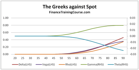
Figure 1 Delta, Gamma, Vega, Theta & Rho for a Deep out of money Call Option

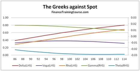
Figure 2 Delta, Gamma, Vega, Theta & Rho for At and Near Money Call Option

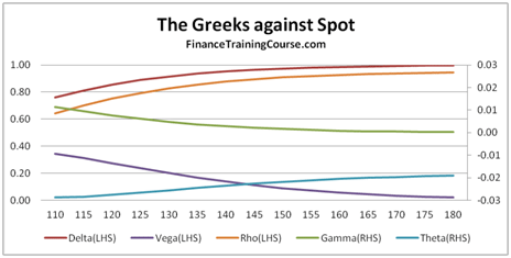
Figure 3 Delta, Gamma, Vega, Theta & Rho for a Deep In Money Call Option


Greeks – Option Price Sensitivities – Formula Reference and one liner definition guide

The five derivative pricing and sensitivities (aka Greeks) with their equations and definition reference

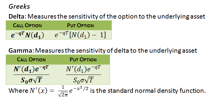
Figure 4 Option Greeks: Delta & Gamma formula reference

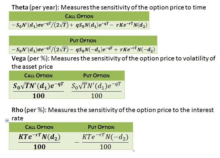
Figure 5 Option Greeks – Vega, Theta & Rho, formula reference

Option pricing – Greeks – Sensitivities – Suspects Gallery

Greeks Against Spot Prices. Here is the short series for Deep out of Money Call Option and Deep In and Out of Money Put options.

Figure 6 Deep out of money call options – Greeks plot

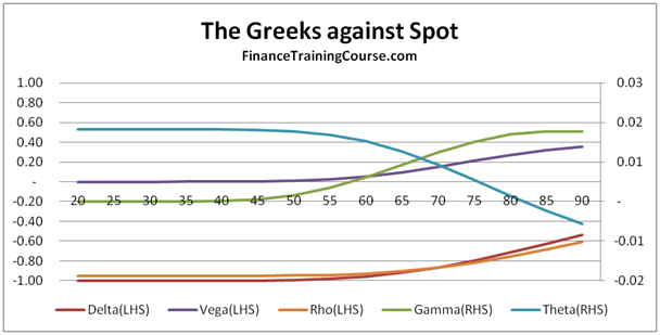
Figure 7 Deep In money put options – Greeks plot

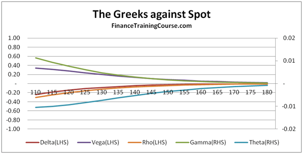
Figure 8 Deep out of money put option – Greek plot

The way to read the above graphical set is to take one Greek at a time. So starting with Delta you will see that while the shape is the same, the sign is different between the Call and the Put. For illustration we have also produced the Greek plot for a Deep out of money Put option and while there are some similarities between the Deep out of money Call and the Deep in money Put, they disappear completely when we look at the Deep out of money Put contract.

Option Price Sensitivities – Plotting Greeks against changing volatility

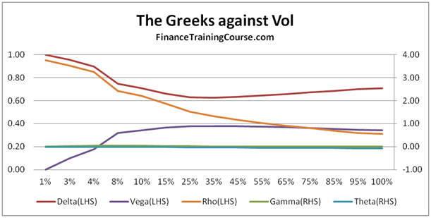
Figure 9 At money Call option – Greek Plot against changing volatilities

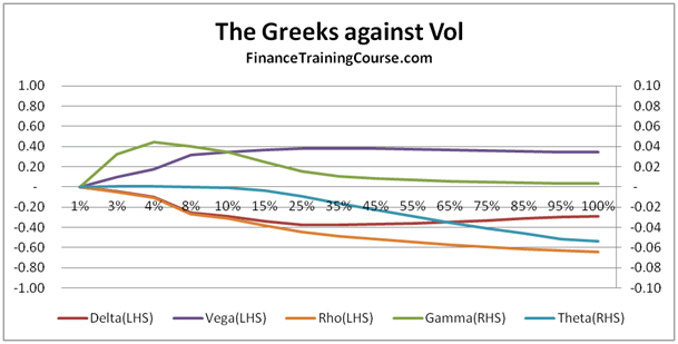
Figure 10 At money put option – Greek plot against changing volatilities

However the difference really crops up between Calls and Puts when you switch the frame of reference from changing spot prices to changing volatilities. With this new point of view Calls and Put are clearly different animals. Why is that? Or is that really the case? If you look closely you will see that as far as Vega, Delta and Rho are concerned the basic shape and shift is similar, it looks different because the LHS axis has shifted. Still Delta is different because of the sign change. But its Gamma and Theta that are really different when it comes to dissecting the behavior of Greeks across Calls and Puts. But would these differences stay if you plot the 5 Greeks across money-ness?

Option Pricing Sensitivities – Greeks – An alternate dimension

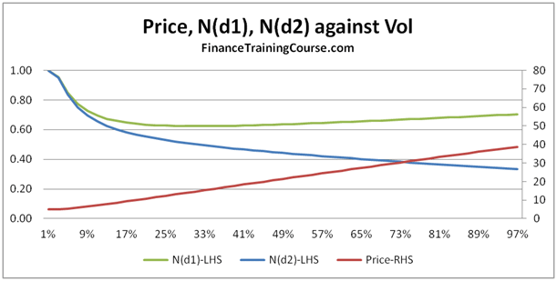
Figure 11 Plotting N(d1), N(d2) and Price against volatility

What do you think is the most common question most students have when they see figure 9 above? Do you see a contradiction? Need a hint? Take a look at Delta. Then think about how we calculate Delta for a European call option. We look at N(d1) as a conditional probability? Intuitively speaking what should we expect N(d1) to do as volatility rises? Rise or Fall? What is N(d1) doing in Figure 9 above?

Now take a look at figure 11 above? What are N(d1) and N(d2) doing as volatility rises? Is that intuitive or counter intuitive? Need a hint? Two words – volatility drag.

Think about the above question and tell us about your answers through the comment sections below in this post. Would love to hear more from you.

Related posts:

  1. Sales & Trading Interview Guide: Understanding Greeks: Option Delta and Gamma
  2. The Sales and Trading Interview Guide Series – Understanding Greeks and Delta Hedging – Coming soon to an iPad near you…
  3. Online Finance – Option Terminology Glossary – Greeks, exotics and volatility

A brew of Volatilities – Implied volatilities, a simplified illustration

This post needs an understanding of the Black Scholes option pricing model (Black Scholes pricing reference). We will discuss at a very simplistic level:

  • Implied volatility
  • Volatility smile

Implied Volatility – Background

In the Black Scholes Merton option pricing framework all parameters are generally known and reasonably stable other than expected future realized volatility. In the academic world we are happy with using historical or empirical volatility as a proxy for future realized volatility but that doesn’t work on a trading desk.

Implied volatility is one way of calibrating option pricing models based on market prices and using market expectations of future volatility rather than historical volatility.

The process for finding implied volatility is the reverse of pricing an option; take the market price of an option, then derive the implied volatility from that price. In other words, now that we know the output, arrive at input volatility using this market price. Hence the name implied volatility.

For our discussion we will consider in-the-money, out-of-money and at-the money options.

Implied volatility – a simple case – calculating implied volatility using excel

We start with out of money call options with one year to expiry. Assume we have the following inputs:

Figure 1 – Implied volatility using excel – Inputs

Note that r, q and T will remain the same for all the cases. We are interested in just changing the stock price at time zero S0 and the strike price k and then use the market price to arrive at the implied volatility.

The volatility box is shaded black because we are still in the dark as to its value.

For this set of inputs, the market price of call option is $18. Now we utilize the excel function of ‘Goal seek’. What is the volatility that will be generate a Black Scholes price of $18? The image below shows the Goal seek setup


Figure 2 – Using Goal Seek to calculate implied volatility

Go to Data tab in Excel, then ‘What-if’ Analysis and then select Goal Seek. Currently value of the call is $4 for a given volatility. However we want to set this equal to $18 by changing cell D7 which is volatility. Press ok.

Figure 3 – Implied volatility using excel – result of the Goal Seek

The Goal seek result is an implied volatility of 60%.

Using the same goal seek function and the approach specified above we attempt to fill the following table:

Figure 4 – Implied volatility – unfilled table

Note that the price is shaded pink and already filled in. This means that the price is not calculated but taken from traders for a call option with respective strike and spot price at time zero.

Using the goal seek function 4 times, the table is filled and shown below:

Figure 5 –Implied volatilities – filled table

Introducing the Volatility smile

Now plot the implied volatility by keeping strike price k as the x-axis.

Figure 6 –Volatility smile

See this curve which looks like a smile? This is the volatility smile. How do we interpret this?

Volatility smile is the observation that an at-the-money options exhibits lower implied volatility than deep out-of-the-money and deep in-the-money options.

Volatility smile is the hole in the constant volatility assumption of Black Scholes. It came to prominence after the 1987 stock market crash.

The journey to modeling volatility smile

The first work was of Hull and White that took ‘stochastic volatility’ as the solution for the smile problem. However, this required a second parameter to be calculated which could not be observed directly, i. e, the market price of volatility risk. The model was also not arbitrage free.

The same challenge applies to jump-diffusion models. This family of models also introduced other parameter(s) that were not observable directly.

Derman and Kani utilized the binomial method. This does not introduce another unobservable parameter and the emphasis in on fitting the data. Another factor lambda is introduced which is calculated as per market prices. Using Arrow-Debreu prices with a binomial tree leads to implied tree .Implied trees result in market consistent prices for plain vanilla as well as exotic options. The Derman Kani model for implied volatility is also arbitrage-free.

However Paul Wilmott criticizes the binomial method calling it a ‘dinosaur’ that takes too much time to yield results.

Other quants look at volatility smile problem in a different manner. The existence of volatility smiles contradicts the normality assumption of Black Scholes as well. The main culprits are skewness and kurtosis. This means that the distribution is more ‘peaked’ at the mean and has thicker tails. Adjustment terms in the Black Scholes are added to account for kurtosis and skewness.

Implied volatilities: Models on models

The main short coming of all the models is that although these theoretical models are consistent with the smile, the statistics and facts show that the smile is about twice as large as predicted by these models; something else is going on.

Ongoing research shows that trading costs are largely to blame for this. Picturing an individual security’s returns with the relative market context and the uncertainty associated with it also causes concerns relating to the shape of the implied volatility.

Implied Volatilities. Conclusion

There is still much research needed before we can reach a solid conclusion as to how to precisely model volatility smile. The common thread researches share however is that there are monetary aspects like trading costs responsible driven by market participant behavior.

Sources

http://202.112.126.97/jpkc/jrysgj/files/18.Why%20do%20we%20smile%20On%20the%20determinants%20of%20the%20implied%20volatility%20function.pdf

http://www.ederman.com/new/docs/gs-volatility_smile.pdf

Related posts:

  1. Financial Risk Management Workshop – Value at Risk, Volatility and Trailing correlations – Day One
  2. Advance Risk Management Models – Workshop & Training reference page
  3. Forwards and Swaps: Interest Rates Models: Bootstrapping the Zero curve and Implied Forward curve