Setting Stop Loss Limits – limit review triggers and back testing. In our case study on setting stop loss limits we reviewed stop loss limit estimates for Oil, Gold and Silver futures trading. In this post we will take a look at market based triggers that should lead to a review of stop loss limits.Changing Volatility Frequency […]
Tag: Sales & Trading Interview Guide
Sales & Trading Interviews – Understanding Greeks & Delta Hedging – Now in Stores
Technical Sales & Trading Interviews – Understanding Greeks & Delta Hedging

Delta Hedging – Designed for audiences with:
- Job Interviews with Sales & Trading, Risk Management or Quantitative Strategies Desks.
- Deadlines for building, tweaking an inhouse dynamic delta hedging model for internal reporting, analysis and discussion.
- Training classes with fresh intake or interns who need to learn the ropes as of yesterday.
- Educating clients & bosses by testing and simulating scenarios cutting across strikes, spots, volatility, rates and time to expiry.
What does it include:

- A Delta Hedging Excel Monte Carlo simulation using our step by step, easy to follow, guide.
- A guide to Simulating Cash PnL for hedging your European Call & Put Exposure
- An analysis of PnL relationships and Option price sensitivities (Greeks)
- Plots of Greeks against changing spot, strike, volatility, expiry & interest rates.
And
- A downloadable 70 page PDF guide for building the Delta Hedging Monte Carlo Simulation in Excel.
- A Greeks suspects gallery for common plots of Delta, Gamma, Vega, Theta & Rho.
- Step by step cash PnL calculation for a Call Option.
- A dissection of Delta, Gamma, Vega, Theta & Rho that doesn’t rely on the formula but uses graphs, intuition and thought experiments.

Understanding Greeks and Delta Hedging – Origins
What started off as a study note to address an intelligent question from a student and completely inadequate teaching on my part, turned into a monster side project that consumed the best part of a year.
The original question dealt with the behavior of Greeks, usage of higher order Greeks by traders and the concept of Delta hedging. It was supplemented by a request for recommended reading that I would care to suggest on this topic.
The challenge was that other than Nassim Taleb’s Dynamic Hedging there is literally nothing out there that you could refer a curious soul to. While Dynamic Hedging is the one and only guide on this topic, it generally leads to Cardiac infractions and CVA’s (Cerebrovascular Accident, not Credit Value Adjustments) in new students. To reduce mortality rate of fresh intakes in computational finance graduate programs and sales and trading desks, there was need for a beginners guide. Ideally with no stochastic calculus and no partial differential equations.
The end result: A study guide that walks through Option Price Sensitivities and Greeks behavior, helps you plot the same in Excel, use a dynamic Delta hedging simulation to get you comfortable with the majors and uses a Cash PnL simulation to dissect the minor Greeks.
It is not a conventional interview guide with interview questions. More like a survival kit that you can use to brush up on Greeks in a rush before the interview or before your exam. You don’t want to digest Taleb the night before; but you can play with an Excel sheet and tweak it to till you are able to connect the missing dots.
The complete package includes a 73 page study note and 3 Excel spreadsheets that you can cover end to end in about 3 hours and build intuition that can help you navigate trick questions and traps in the interview room.
![]()

Pick a copy under the early buyers promotion valid till 3oth November and take $60 dollars off the cover price.
Understanding Option Greeks – Free Sample content
The problem with Greeks is that the topic is so out there for most students and non-practitioners that we would rather ignore it. Who would actually care about the second moment (Gamma) or the third (Delta of Gamma) for that matter in the non-trading desk world. Plus by the time you actually get to a level that you can talk intelligently about the subject you are so short of oxygen that there is nobody left to talk to.
Understanding Greeks – Introduction
Understanding Greeks – Analyzing Delta & Gamma
Understanding Greeks – The Guide to delta hedging using Monte Carlo Simulation
Dynamic Delta Hedging Simulation – Cash PnL calculations
Using Dynamic Delta Hedging Simulation as a learning tool
Understanding Greeks – Quick Reference Guide to Delta, Gamma, Vega, Theta & Rho
Understanding Greeks & Delta Hedging – Motivation
I remember the pain I went through when I first tried to decipher Greeks, Continuous Time Finance and Monte Carlo Simulations. It was only when I met Mark Broadie and Maria Vassalou at Columbia that the cobwebs in my mind cleared up. While this book doesn’t deal with the original pain, it uses the approach Mark used to teach us a fairly difficult subject. Use Excel, Monte Carlo Simulation and intelligent questions (aka thought experiments).
The book is therefore packaged with spreadsheets that can be used interactively with relevant sections (see included Excel spreadsheets detail specification at the end of this post). As a student you can actually build the sheets using the step by step guides or simply use the packaged editions to answer the questions we ask.
And we ask many questions. In fact in one specific section we lead you all around town using the incorrect approach till you finally figure out the right answer. I have found this to be one of the most effective ways of ensuring comprehension and understanding.
The 73 pages are primarily a guide to building a delta hedging spreadsheet for European Call and Put Options. Nassim Taleb emphasizes the use of a generator function to build trader intuition and we have included one. We then use the Delta hedging sheet to think about Delta, Gamma, Vega & Rho by asking questions that help reinforce that intuition. For Greeks we include an Excel calculation spread sheets as well as over thirty graphs that analyze Greeks behavior across changing Spot, Strikes, Volatility, Time & Interest rates.
To get the most out of the package, we recommend that you follow the book and the templates to build your Excel spreadsheets from scratch.
However the most important section of the book deals with Cash PnL from dynamic hedging. It turns out to be a terrific tool, once you link the profitability calculation to Greeks and use it to dissect components and contributors to PnL.
The Table of Content produced below has more details.
Pick a copy under the early buyers promotion valid till 30th November and take $60 dollars off the cover price.
Dynamic Delta Hedging – Monte Carlo Simulation – Greeks – Downloadable Excel File Guide
This product contains 3 EXCEL files.
1. Option Greeks Calculation & Graphs
- Calculation of the Black Scholes option price for a European Call and a European Put option
- Calculation of Greeks- Delta, Gamma, Vega, Theta & Rho- for a European Call and a European Put option
- Data table that captures the Black Scholes risk adjusted probabilities and option premium across a series of volatilities
- Graphical representation of Black Scholes risk adjusted probabilities and option premium against volatilities
- Data tables that capture the sensitivity of the Greeks against Spot, Strike, Time to maturity, Volatility and the Risk Free Rate respectively
- Graphical representation of the sensitivities of the various Greeks against Spot, Strike, Time to maturity, volatility and risk free rate respectively
2. Dynamic Delta Hedging – Call Option – Monte Carlo Simulation – Cash PnL
- Calculation of a 12-step Monte Carlo simulation model that generates the underlying stock price series
- Calculation of theoretical option values using the Black Scholes call option price formula
- Calculation of call option deltas at each rebalancing interval
- Calculation of a replicating portfolio that consists of a long position in Delta times the stock and a short position in the amount borrowed (net of the option premium received at inception) to fund the initial & subsequent incremental purchases
- Graphical representation of the theoretical option value and the replicating portfolio value over the life of the option
- Calculation of a tracking error for the difference between the value of the replicating portfolio and the theoretical value of the option
- Graphical representation of the tracking error across the life of the option
- Determination of the per period interest and principal portions of the amount borrowed
- Determination of the Gain (Loss) on sale of portions of the stock
- Setting up a Cash Accounting P&L that shows cash inflows from option premium received and strike received in the event the option is exercise and cash outflows from interest and principal repayment on the amount borrowed
- A choice of including of excluding the option premium in determining the amount borrowed at inception. In this case the Principal repaid will equal the gain (loss) if the option is not exercised.
- 100 simulated runs including a graphical depiction of the results showing the Net P&L, Amount borrowed (principal & interest) and Gain/ Losses; and averages across the 100 runs for each of these items
3. Dynamic Delta Hedging – Put Option – Monte Carlo Simulation – Cash PnL
- Calculation of a 12-step Monte Carlo simulation model that generates the underlying stock price series
- Calculation of theoretical option values using the Black Scholes put option price formula
- Calculation of put option deltas at each rebalancing interval
- Calculation of a replicating portfolio that consists of a short sale of Delta times the stock and lending of the initial (net of the option premium received at inception) & subsequent incremental short sales proceeds
- Graphical representation of the theoretical option value and the replicating portfolio value over the life of the option
- Calculation of a tracking error for the difference between the value of the replicating portfolio and the theoretical value of the option
- Graphical representation of the tracking error across the life of the option
- Determination of the per period interest and principal portions of the amount lent
- Determination of the Gain (Loss) on closing of short sale positions
- Setting up a Cash Accounting P&L that shows cash inflows from option premium received, interest earned on amount lent and sales proceeds from short sales and cash outflows from strike paid if the option is exercised
- A choice of including or excluding the option premium in determining the amount borrowed at inception. In this case the sales proceeds from short sales will equal the gain (loss) if the option is not exercised.
- 100 simulated runs including a graphical depiction of the results showing the Net P&L, Proceeds from Short Sales, Interest Earned and Gain/ Losses; and averages across the 100 runs for each of these items
![]()
Pick a copy under the early buyers promotion valid till end of November and take $60 dollars off the cover price.
Related posts:
Delta Hedging applications for Rho, Rebalancing frequency & Implied Volatility
Rebalancing frequency, Implied Volatility & Rho. Dynamic Delta Hedging Applications.
Now that we have a Delta Hedging Model for Calls and Puts let’s try and use it to answer the following questions:
a) What is the impact of rebalancing frequency on hedging profitability?
b) What is the impact of a rise in volatility on profitability? How does implied volatility help in interpreting this change?
c) What is the impact of changes in risk free rates on profitability?
d) How does the interaction of time to expiry and volatility changes profitability?
These are all questions that should occur naturally to you as you spend more time with the Delta Hedging model. They are also essential to building a deeper understanding of the concept of implied volatility, Rho & Theta.
Dynamic Delta Hedging Questions: Assumptions & Securities
Let’s take a look at these questions one by one. We will begin work with a call option assuming the following valuation parameters:
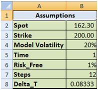
Figure 1 Dynamic Delta Hedging – P&L review assumptions
The theoretical value of the call option is 3.01 based on the above assumptions. The resulting Cash Accounting P&L for a single run of the Dynamic Delta Hedging model is as under:
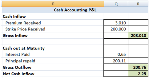
Figure 2 Dynamic Delta Hedging – P&L Review – Base case
Rebalancing frequency & efficiency of the hedge. Implications for profitability?
A good hedge is one where the cost of the hedge is close to the theoretical value of the option. In our cash accounting P&L we have included the theoretical premium received which is used in determining the initial amount to be borrowed. Hence for a hedge to be considered good or efficient the Net P&L should be close to this premium amount.
To see if increasing the frequency led to better results, we increase the time steps used from 12 steps to 365 steps. The graph below plots the Net P&L to Theoretical Value across 100 simulated runs. A value close to 100% means that it is a close match to the premium whereas a value farther away for 100% indicates a poor match.
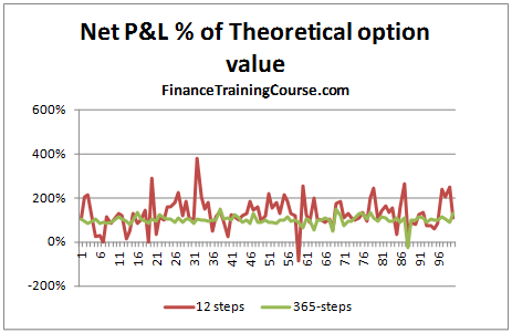
Figure 3 Dynamic Delta Hedging – P&L Simulation – Rebalancing frequency
We can clearly see that there is much greater variation when the rebalancing is done on a monthly basis than when it is carried out on a daily basis.
The graph below gives a similar picture. In this case however, the premium is not considered when determining the amount to be borrowed at option inception, i.e. the hedge is fully funded through borrowing. A value of -100% indicates that the Net P&L i.e. the cost of the hedge, in this case exactly matches the theoretical value of the call option.
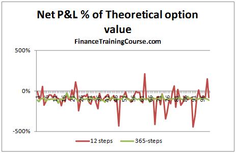
Figure 4 Dynamic Delta Hedging – P&L Simulation – Hedge Effectiveness
But that is the risk manager’s point of view. What about a trader’s point of view?
From a trading point of view there are two lessons here. First the large variation in P&L linked to jump’s in the underlying price is the un-hedged Gamma at work (Is that true? Think about it). Second would you prefer to limit the cost of hedging the option to the amount you have charged your customer or less? If you are in the business of earning a living from writing options, the premium you charge on the options you sell should always be higher than your cost; your cost of effectively hedging the option.
Now back to the Gamma question. Gamma is your second order error term. Conceptually it’s similar to convexity and linked to changes in not just the underlying price but also volatility. Is your true P&L (the premium received less the actual cost of hedging) is the summation of the hedge error?
Volatility and profitability. The question of implied volatility
With volatility there are multiple questions. How does profitability change when the general environment moves from low volatility to high volatility? How does profitability change when you have already written an option and volatility moves for or against you?
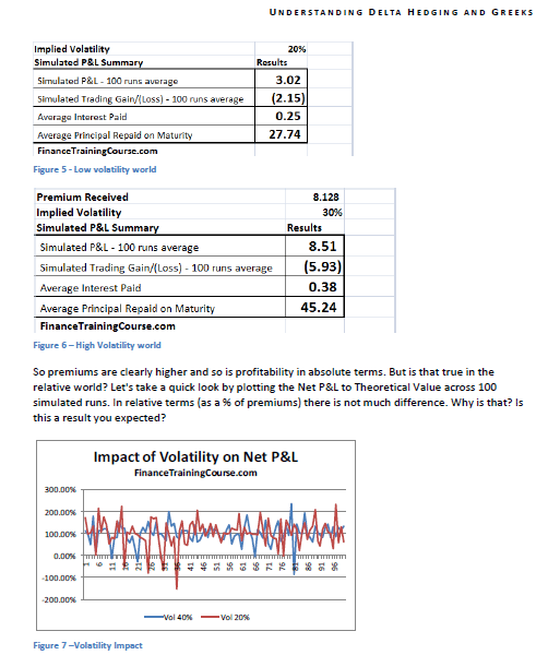
Let’s start from the first question. Using the 12-step model we calculate the impact on Net P&L. In our base case we have assumed a volatility of 20%. Let us now assume that the volatility increases to 40%. What is the impact on hedge efficiency for options written in the two different environment?
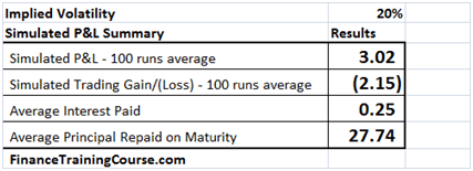
Figure 5 Volatility & Profitability – Low volatility world
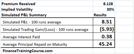
Figure 6 Volatility & Profitability – High Volatility world
So premiums are clearly higher and so is profitability in absolute terms. But is that true in the relative world? Let’s take a quick look by plotting the Net P&L to Theoretical Value across 100 simulated runs. In relative terms (as a % of premiums) there is not much difference. Why is that? Is this a result you expected?
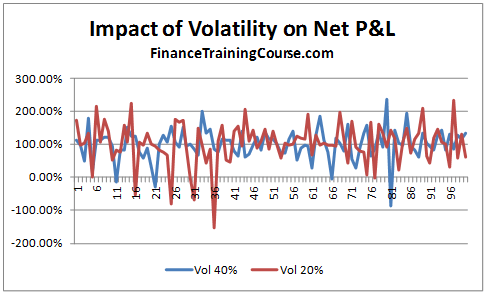
Figure 7 Dynamic Delta Hedging – P&L Simulation – Volatility Impact
To answer these questions you have to revisit implied volatility. Let’s use the same scenario as above but with a minor change. We wrote options and received premiums assuming an implied volatility of 30%. The actual realized volatility over the life of the option was 20%. How did that change our resulting simulated P&L.
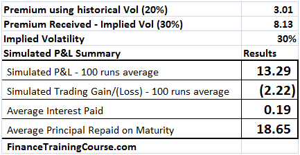
Figure 8 Implied volatility at work – Hedge Profitability
You can now see a clear difference in absolute as well as relative terms in net P&L. And the difference arises on account of the spread between the premium charged ($8.13) versus the premium needed ($3.01).
(To run this exercise using the Delta Hedge Sheet, simply calculate the value of the premium at the implied volatility level you want to charge and replace the original premium in the simulation with this value).
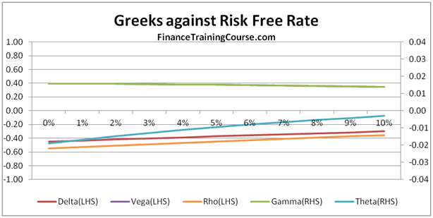
Risk free rates & profitability. The question of Rho.
We present the results of three P&L simulations runs in the tables below. The first assumes a risk free interest rate of 1%, the 2nd uses 2% and the third uses a risk free interest rate estimate of 5%.
The first two are easy, rates go up, premiums goes up and a European Call option becomes more expensive. Why is that?
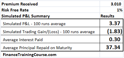
Figure 9 Dynamic Delta Hedging profitability – P&L at 1% interest rates
The reason is the average interest paid column. The premium goes up by 28 cents of which 21 cents is the increased cost of financing the borrowed position. Where does the other 7 cents comes from? (Need a hint – Other than the borrowing component who else benefits or uses r, the risk free rate?)

Figure 10 Dynamic Delta Hedging profitability – P&L at 2% interest rate
The second one is more difficult. In this instance as rates increase to 5% from the original 1%, the cost of borrowing balloons to $1.95 from the original $0.30 but the impact in option premium is only $1.244. How does this work? (Hint, think about what other driver/factor in the Black Scholes Analysis uses r?)
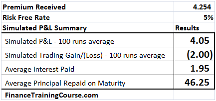
Figure 11 Dynamic Delta Hedging profitability – P&L at 5% interest rates
In addition to borrowing the difference between premium received and Delta hedge, the other usage of the risk free rate, r, is in estimating the future value of the underlying asset in the BSM (Black Scholes Model’s) risk neutral world. This implies that there are other components of Rho, in addition to the borrowing cost. That you need to examine and be comfortable with.
Related posts:
Hedging Gamma & Vega – The higher order Greeks hedge optimization Excel spreadsheet – Part I
Hedging Higher Order Greeks – Hedging Gamma & Vega using Microsoft Excel
In earlier posts we have set the foundation for hedging in practice. We did this by calculating Option Price Sensitivities (Greeks) and Delta hedging for European Call as well as Put Options.
Why would you want to hedge Gamma?
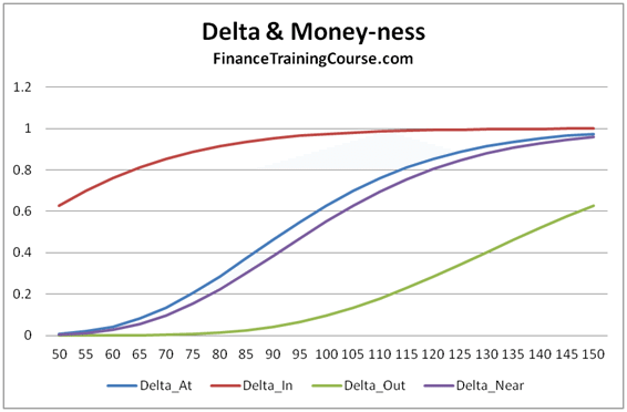
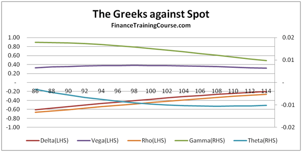
Figure 1 Options Greeks – Delta and Moneyness – Hedging higher order Greeks
If you leave it un-hedged you are exposed to the risk of large moves, especially when the option is at or near money. When you are deep out or deep in, Delta is flat and asymptotic as shown above. But when are you not, a large move can result in significant trading loss despite being Delta hedged. As long as prices move in small increments and do not jump dramatically, Delta hedge will cover you. The underlying jumps, you are exposed.
We have seen this at work earlier with duration and convexity with similar implications. Delta is the first order rate of change and works well within a narrow band. Within and outside that band Gamma tracks not just the error but also the magnitude of your gain/loss in case of a large move (up/down). The magnitude of the error shifts dramatically as the option gets closer to the At/Near money state. When options are deep in or deep out, similar to Delta, Gamma also flattens out. However given the convex nature of the 2nd derivative in this case, the impact of a large up move or a large down move is not symmetric.
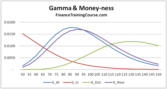
Figure 2 Option Greeks – Gamma & Moneyness – Hedging Higher order Greeks
But you can’t hedge higher order Greeks (Gamma) by buying or selling the underlying. Why not?
First the 2nd derivative of a spot/forward/linear position is zero so hedging Gamma through the underlying is out. The second complexity arises with Vega. We really don’t know what shape or form realized volatility will take in the future. How can we effectively hedge it?
Then there is the issue of term structure of volatility. Implied volatility changes based on time to maturity (term structure) as well as money-ness (deep in, deep out, At/Near – strike price) so taking a simple constant volatility view across all options irrespective of maturity or money-ness would actually be in-accurate.
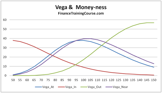
Figure 3 Option Greeks – Vega & Moneyness – Hedging higher order Greeks
The third catch is that both Gamma and Vega use exactly the same calculation function for Calls and Puts (Gamma for a call and put has the same value, Vega for a call and a put has the same value). Which creates interesting implications for hedging a book of options with calls and puts. You may be perfectly hedged and squared with respect to your Gamma and Vega exposures but the wrong universe/direction of hedging choices can still wipe you out.
We hedge Gamma and Vega by buying other options (specifically cheaper out of money options) with similar maturities. Like Delta hedging we need to rebalance but the rebalance frequency is less frequent than Delta hedging. Your final hedge is therefore a mix of exposure to the underlying (partial delta hedge) and cheaper options with similar maturities.
The only question is that it’s a large universe of options out there, how do we manage multiple constraints including premium & sensitivities across products, maturities (tenors), Delta, Gamma & Vega. The answer is constraint optimization through Excel solver. In our next post we will show how to build a simple Excel solver model that takes a universe of four options and uses it to match the required Delta, Gamma, Vega profile for a single option.
Before we jump to the next post, please review the following background posts on Option Greeks & Delta Hedging to ensure that you are comfortable with the calculation of Delta, Gamma & Vega as well the implementation of Delta Hedging in Excel.
Understanding Option Greeks – Relevant Sales & Trading Interview Guides posts
Understanding Greeks – Introduction
Understanding Greeks – Analyzing Delta & Gamma
Understanding Greeks – The Guide to delta hedging using Monte Carlo Simulation
Understanding Greeks – Quick Reference Guide to Delta, Gamma, Vega, Theta & Rho
Related posts:
Sales & Trading Technical Interviews – Greeks behaving badly – Put Options
Understanding Option Price Sensitivities – European Put Options – Sales & Trading Technical Interview Guides
As part of our Sales & Trading technical interview guide series we have done a number of posts on Greeks, Delta hedging and estimation of Delta hedging Profit & Loss.
A recent client/student/interview request indicated a preference/need for a sheet dedicated to European Put Options Greek plots. Hence the Greeks Put Option suspects’ gallery. While some of these are making a second appearance, we think a Put only collection is indeed useful given our focus on European Call options.
The Analysis framework used for dissecting put option Greeks is simple. We break the contracts down by “money-ness”. The three categories are Deep In, At/Near, Deep Out of money options.
And the five option pricing variables – Spot, Strike, Vol, Interest Rates & Time. This analytical combination produces interesting results.
The options for which Greeks have been plotted below assume a volatility of 20%, a risk free rate of 5% and a time to maturity of 1 year. In addition Spot and Strike prices are:
Deep In
Spot = 50
Strike = 100
At/Near
Spot = 50
Strike = 100
Deep Out
Spot = 50
Strike = 100
Greeks Against Spot – European Put Options
European Put Options – Deep In the money Options
European Put Options – At/Near Money Options
European Put Options – Deep Out of money Options

Greeks Against Spot – European Put Options
European Put Options – Deep In the money Options
European Put Options – At/Near money Options
European Put Options – Deep out of money Options
European Put Option Greeks – Against Volatility
European Put Options – At/In money Options
European Put Options – Against Changing Interest Rates
European Put Options – At/Near money Options
European Put Options – Against Changing Time to Maturity
European Put Options – At/Near money Options
Understanding Option Greeks – Relevant Sales & Trading Interview Guides prior posts
Understanding Greeks – Introduction
Understanding Greeks – Analyzing Delta & Gamma
Understanding Greeks – The Guide to delta hedging using Monte Carlo Simulation
Understanding Greeks – Quick Reference Guide to Delta, Gamma, Vega, Theta & Rho
Related posts:
Dynamic Delta Hedging – Calculating Cash PnL (Profit & Loss) for a Call Option writer
Dynamic Delta Hedging – Calculating Cash PnL (P&L) for a European Call Option
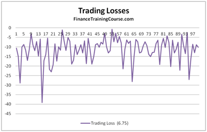
Figure 1 Delta Hedge P&L – Trading losses on account of rebalancing
We extend the original Dynamic Delta Hedging Monte Carlo Simulation spread sheet in this note. The dynamic hedging spreadsheet for a European call option allowed us to do a step by step trace of a delta hedging simulation. In this sheet we will use the results from the simulation trace to calculate a cash accounting P&L for our hedging model assuming the role of a call option writer and then extend the original simulation to see the average PnL across 100 iterations.
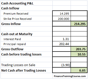
The above calculation has a double count in it? Which directly impacts the final profitability figure? Can you see it? See the discussion below for an answer.
We are assuming that we have written a European call option on Barclays Bank where the current spot price is $162.3 and the strike price is US$200. Time to expiry is one year and Barclays Bank is unlikely to pay a dividend during the life of the option.
Figure 2 Delta Hedge P&L – Cash P&L for the writer for a call option that expires in the money
Understanding Delta Hedging Cash PnL Calculation – Required resources
Before you proceed further if you are still uncomfortable with option price sensitivities or delta hedging please use the following background and model review posts to make yourself comfortable with the underlying concepts.
- Understanding option Greeks reference resource for dummies
- Understanding Greeks – Analyzing Delta & Gamma
- Understanding Greeks – The Guide to delta hedging using Monte Carlo Simulation
- Understanding Greeks – The Delta Hedging Simulation extended for Put Options
Delta Hedging Cash PnL Calculations – Dissecting the PnL Model
Our model uses a simplified cash based approach to calculate PnL from our Delta Hedging model. Our objective is to calculate PnL at option expiry for the option writer. Primary contributors to the model include:
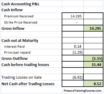
Figure 3 Delta Hedge – Cash P&L for the writer for an option that expires out of money
a) Cash in – receipts from the customer. Include premium received and the strike price if the option is exercised. If the option expires worthless we only receive the premium.
b) Cash out. As explained earlier to finance our hedge purchases we borrow money. We pay interest on this principal for the life of the hedge and return the principal at maturity.
c) Trading losses. As part of our strategy we purchase the underlying as prices rise and sell it when they fall. Be definition this strategy will generate trading losses irrespective of whether the option expires worthless or in the money. Because we re-balance on a frequent basis, trading losses also consume cash. However the question that often confuses audiences is one of double count. Should trading losses be included as a separate accounting item or are they already included in the Cash before trading losses calculation? Think about this before you proceed further. It will directly impact your analysis and result. Here is a hint – other than the cash treatment that we have used, is there any other possible use or source of cash in the analysis and the calculation above?
When we put the model in place our final output should look something like this:

Figure 4 Delta Hedge P&L Simulation results – Gross P&L, Net P&L, Trading Losses
You can clearly see that the biggest contributor to our cash PnL uncertainty is trading loss. Is this treatment correct?
We will take a more closer look at this contributor later in our note.
Extending the Delta Hedge Model for Cash PnL Calculation – Interest paid & principal borrowed for the Hedge
The first step is to add two new columns to our Delta hedge model. These are:
- Interest paid per period, and
- Incremental amount borrowed per period
Both elements have been calculated as part of the original sheet and all we need to do is simply extract the relevant piece and dump the results in two new columns at the end.
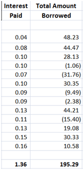
Figure 5 Delta Hedging PnL – Two new columns – Interest paid & Marginal borrowing
Incremental amount borrowed is included in the total borrowing figure we had calculated earlier in the Guide to delta hedging using Monte Carlo Simulation
post. It is simply the difference between the two deltas for the two time periods multiplied by the new price of the underlying stock.
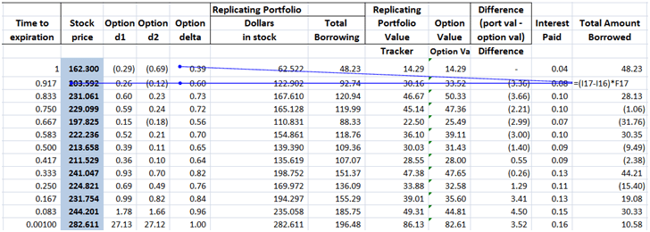
Figure 6 Delta Hedging PnL – Calculating Incremental borrowing
Interest paid per period is the interest accrued on the balance of the previous period. Which ends up as outstanding balance times the interest accrual factor (exp(risk_free_rate x Delta_T)) in the sheet.
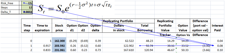
Figure 7 Delta hedging PnL – Calculating Interest paid on borrowed cash
Delta Hedging PnL – Calculating the trading loss on account of selling low
The basic hedging strategy is to buy when delta (or price) goes up and sell when delta (or price) goes down. Buy when prices rise, sell when they decline. The result is that as the underlying price see-saws, we end up buying high and selling low, rebalancing the portfolio in alignment with delta but also generating trading losses.
Our calculation of trading losses has three components.
a) First calculate the number of incremental units purchased or sold as part of the required rebalancing. (Unit purchased column)
b) Then calculate the difference in price between the two rebalancing periods. (Difference in price column)
c) Finally identify all trades where a sale was made and calculate the trading gain or loss. (Loss on Sale column)
For this specific simulation the trading loss is calculated as $2.5 based on the above approach.
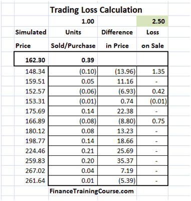
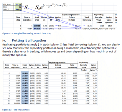
Figure 8 Delta Hedge simlation – trading loss calculation
Delta Hedge PnL Calculation – Putting it all together
Now that we have all of the required PnL components together we hook them up with our Excel Data Table. We use our Monte Carlo bag of tricks to store the results of 100 iterations. Stored components include Gross PnL (excluding trading losses), Net PnL (including trading losses), Interest Paid & Trading loss on rebalancing sales.
But there is a trick question here. Its the question that has always stumped students (and quite frequently me). Here is the question. Is the correct P&L the Gross P&L or the Net P&L figure below? The net P&L subtracts the trading loss from the gross figure. Is that a double count? How would you explain and justify the answer? Is there a one word answer?
Think about these questions as you work through the numbers in the table below. We will do a post answering the double count question later. In the interim period here is a hint. Try a fully funded (zero premium) strategy once you have built the sheet and see what happens to your P&L calculation.
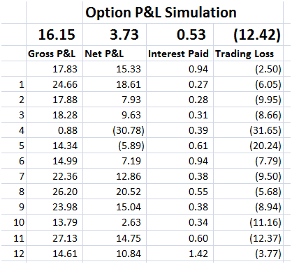
Figure 9 Delta Hedge PnL – Storing the results
(If this doesn’t make sense, take a quick look at our Monte Carlo Simulation refresher below.)
The final result is our Delta Hedge PnL graph for a European Call Option.
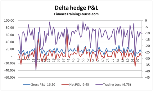
Figure 10 Dynamic Delta hedge PnL Calculation – PnL Graph
Delta hedging PnL – Next steps and Questions
Once you have the basic model figured out here are some interesting questions that follow:
a) How would you extend this model for PnL calculations for a European Put Option?
b) How would you incorporate the impact of implied volatility?
c) Of transaction costs? And non-risk free interest rates? Jumps and Dividends?
d) How would profitability (cash PnL) change if you shortened the time step and the rebalancing period? Or extended it?
e) What does the distribution of profits suggests about the risk inherent in the underlying business?
f) Is this the most effective way of hedging options?
g) What about the risk embedded in other Greeks? How is that managed and hedged? How does that impact PnL?
Related posts:
Advance Risk Management Models – Implied volatilities and volatility smile. A simple review
A brew of Volatilities – Implied volatilities, a simplified illustration
This post needs an understanding of the Black Scholes option pricing model (Black Scholes pricing reference). We will discuss at a very simplistic level:
- Implied volatility
- Volatility smile
Implied Volatility – Background
In the Black Scholes Merton option pricing framework all parameters are generally known and reasonably stable other than expected future realized volatility. In the academic world we are happy with using historical or empirical volatility as a proxy for future realized volatility but that doesn’t work on a trading desk.
Implied volatility is one way of calibrating option pricing models based on market prices and using market expectations of future volatility rather than historical volatility.
The process for finding implied volatility is the reverse of pricing an option; take the market price of an option, then derive the implied volatility from that price. In other words, now that we know the output, arrive at input volatility using this market price. Hence the name implied volatility.
For our discussion we will consider in-the-money, out-of-money and at-the money options.
Implied volatility – a simple case – calculating implied volatility using excel
We start with out of money call options with one year to expiry. Assume we have the following inputs:
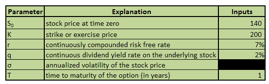
Figure 1 – Implied volatility using excel – Inputs
Note that r, q and T will remain the same for all the cases. We are interested in just changing the stock price at time zero S0 and the strike price k and then use the market price to arrive at the implied volatility.
The volatility box is shaded black because we are still in the dark as to its value.
For this set of inputs, the market price of call option is $18. Now we utilize the excel function of ‘Goal seek’. What is the volatility that will be generate a Black Scholes price of $18? The image below shows the Goal seek setup
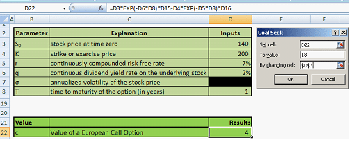
Figure 2 – Using Goal Seek to calculate implied volatility
Go to Data tab in Excel, then ‘What-if’ Analysis and then select Goal Seek. Currently value of the call is $4 for a given volatility. However we want to set this equal to $18 by changing cell D7 which is volatility. Press ok.
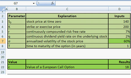
Figure 3 – Implied volatility using excel – result of the Goal Seek
The Goal seek result is an implied volatility of 60%.
Using the same goal seek function and the approach specified above we attempt to fill the following table:
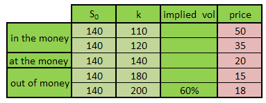
Figure 4 – Implied volatility – unfilled table
Note that the price is shaded pink and already filled in. This means that the price is not calculated but taken from traders for a call option with respective strike and spot price at time zero.
Using the goal seek function 4 times, the table is filled and shown below:
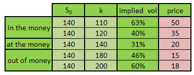
Figure 5 –Implied volatilities – filled table
Introducing the Volatility smile
Now plot the implied volatility by keeping strike price k as the x-axis.
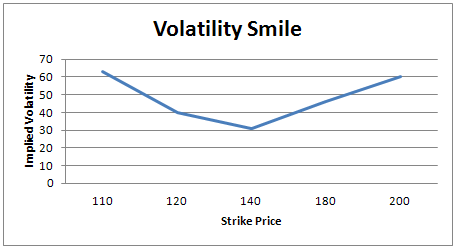
Figure 6 –Volatility smile
See this curve which looks like a smile? This is the volatility smile. How do we interpret this?
Volatility smile is the observation that an at-the-money options exhibits lower implied volatility than deep out-of-the-money and deep in-the-money options.
Volatility smile is the hole in the constant volatility assumption of Black Scholes. It came to prominence after the 1987 stock market crash.
The journey to modeling volatility smile
The first work was of Hull and White that took ‘stochastic volatility’ as the solution for the smile problem. However, this required a second parameter to be calculated which could not be observed directly, i. e, the market price of volatility risk. The model was also not arbitrage free.
The same challenge applies to jump-diffusion models. This family of models also introduced other parameter(s) that were not observable directly.
Derman and Kani utilized the binomial method. This does not introduce another unobservable parameter and the emphasis in on fitting the data. Another factor lambda is introduced which is calculated as per market prices. Using Arrow-Debreu prices with a binomial tree leads to implied tree .Implied trees result in market consistent prices for plain vanilla as well as exotic options. The Derman Kani model for implied volatility is also arbitrage-free.
However Paul Wilmott criticizes the binomial method calling it a ‘dinosaur’ that takes too much time to yield results.
Other quants look at volatility smile problem in a different manner. The existence of volatility smiles contradicts the normality assumption of Black Scholes as well. The main culprits are skewness and kurtosis. This means that the distribution is more ‘peaked’ at the mean and has thicker tails. Adjustment terms in the Black Scholes are added to account for kurtosis and skewness.
Implied volatilities: Models on models
The main short coming of all the models is that although these theoretical models are consistent with the smile, the statistics and facts show that the smile is about twice as large as predicted by these models; something else is going on.
Ongoing research shows that trading costs are largely to blame for this. Picturing an individual security’s returns with the relative market context and the uncertainty associated with it also causes concerns relating to the shape of the implied volatility.
Implied Volatilities. Conclusion
There is still much research needed before we can reach a solid conclusion as to how to precisely model volatility smile. The common thread researches share however is that there are monetary aspects like trading costs responsible driven by market participant behavior.
Sources
http://www.ederman.com/new/docs/gs-volatility_smile.pdf
Related posts:
Sales & Trading Interview Guide: Understanding Greeks: Option Delta and Gamma
Sales & Trading Interview Guide: Understanding Greeks. Option Delta and Gamma.
Here is a short and sweet extract from the Sales & Trading Interview Guide series on Understanding Greeks (iBook and plain vanilla PDF version in the works). Rather than focus on formula and derivations, we have tried to focus on behavior. Our hope is the pretty pictures and colored graphs would help take some of the pain away from comprehending this topic.
Delta, Gamma, Vega, Theta & Rho. The five Greeks
There are five primary factor sensitivities that we are interested in when it comes to option pricing and derivative securities.
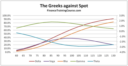
Figure 1 The Five Greeks. Plotted against changing spots
The image above presents a plot of the five factors for an At The Money (ATM) European call option.
Delta (Spot Price)- Measures the change in the value of the option price, based on a change in price of the underlying. Delta is the dark red line in the image above.
Vega (Volatility) – Measures the change in the value of the option price, based on a change in volatility of the underlying. Vega is the dark indigo line in the image above.
Rho (Interest Rates) – Measures the change in the value of the option price based on a change in interest rates.
Theta (Time to expiry) – Measures the change in the value of the option price based on a change in the time to expiry or maturity.
The first four sensitivities measure a change in the value of the option price based on a change in one of the determinants of option prices – spot price, volatility, interest rates and time to maturity. The fifth and final sensitivity is a little different. It doesn’t measure a change in option price, but measures a change in one of the sensitivities, based on a change in the price of the underlying.
Gamma – Measures a chance in the value of Delta, based on a change in the price of the underlying. If you are familiar with fixed income analytics, think of Gamma as Delta’s convexity.
As promised above, we won’t hit you with any equations. However a quick notation summary is still required to appreciate the shape of the curves you are about to see.
Delta, Vega, Theta and Rho are all first order changes, while Gamma is second order change. If you take a quick look at the plot of the five factors presented above, you will see that the shape of the curves are similar for Delta and Rho (the slanting S) and similar for Gamma, Vega and Theta (the hill or inverted U). We will revisit the shape debate later on in our discussion.
Sales and Trading Interview Guide: Let’s talk about Delta
Delta has a handful of interpretations. Some common, some exotic.
The common interpretation is the one we have just covered above. Delta tracks option price sensitivity to changes in the price of the underlying. The second interpretation is as a conditional probability of terminal value (St) being greater than the Strike (X) given that St > X for a call option.
The third and the most relevant definition to our discussion comes from the option replicating and hedging portfolio example from the Black Scholes world.
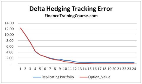
Figure 3 Delta Hedging. Replicating portfolio for call option using option Delta
As a seller of a call option if you would like to hedge your exposure (short call option) so that when (or if) the call option is actually exercised your loss is ideally completely offset by the change in value of your replicating portfolio.
This replicating portfolio is defined as a combination of two positions. A long position in the underlying given by Delta x S, less a borrowed amount.

Figure 4 – The Delta Hedge Relationship
For a European call option Delta is defined as

If we adjust Delta and with it the borrowing amount at suitably discrete time intervals we will find that our replicating portfolio will actually shadow or match the value of the option position. When the option is finally exercised (or not exercised) the two positions will offset each other.
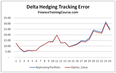
Figure 5 Delta Hedging. Replicating portfolio performance for hedging a short call option exposure
The two replications snap shots shown above show how closely the two portfolios move with changes in the underlying price over a one year time interval with fortnightly rebalancing (24 time steps). The tracking error will reduce if the rebalancing frequency is increased but it will also increase the cost of running the replicating portfolio.
Now that we have gotten the basic introduction out of the way, let’s spend some time on dissecting Delta by evaluating how this measure of option price sensitivity changes as you change:
a) Spot,
b) Strike,
c) Time to expiry and
d) Volatility.
Where relevant and important, we will add more context by also looking at how Delta’s behavior changes if the option is in, at, near or out of money.
Sales and Trading Interview Guide: Dissecting Delta – Against Spot
So how does Delta behave across a range of spot prices.
If we assume that we have purchased or sold a call option on a non-dividend paying stock with a strike price of US$100. The underlying is currently trading at a spot price of US$100. The time to expiry or maturity is one year.
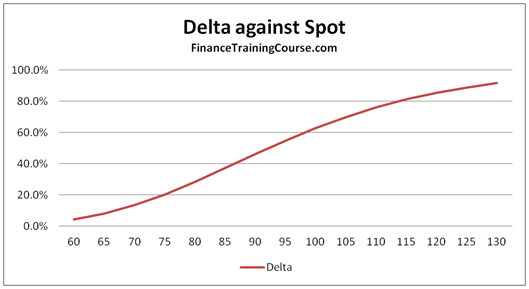
Figure 6 Delta plotted against changing spot prices
The graph above shows the change in the value of Delta as spot prices move higher or lower from the original US$100.
In this specific instance while we have moved spot prices we have held maturity constant. As a result while spot prices for the underlying change from 60 to 130, the option’s delta doesn’t touch zero or 1, since there is a chance that it may still switch direction and go the other way.
How does the behavior of Delta change if you move across At money options to options that are deep out of money or deep in the money? Think about this for a second before you move forward. Would you expect to see a different curve? Or a different shape? How different?
Let’s start with at, in and near money options.
For at money or near money options the shape remains the same. For options that are deep in the money, it becomes asymptotic before finally touching 1. From our hedging definition above, this means that the seller of the option should now own the exact numbers of shares of the underlying committed to the call option (Delta = 1) since the option will most certainly expire in the money. From a probability definition perspective, for a call option a conditional probability of 1 indicates that the option is certain to expire in the money.
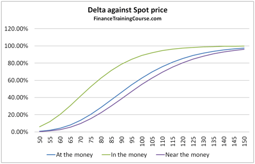
Figure 7 Delta against Spot. At, In and near money options
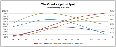
But what about deep out of money options? What happens to Delta or for that matter to all the other Greeks discussed earlier when it comes to deep out of money options.
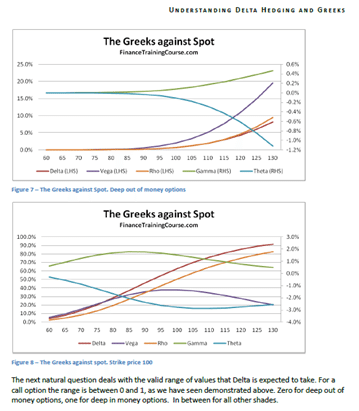
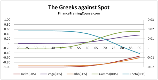
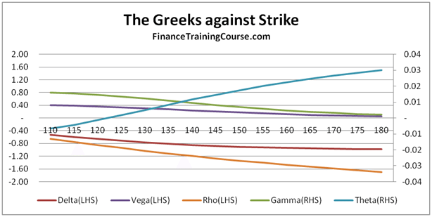
We answer this question by plotting the Greeks for a European call option written with strike price of US$200, while the current spot price is only at US$100. In the price ranging between US$60 and US$130, the value of Delta touches zero and then slowly rises to about 8% as the underlying spot price reaches US$130.
The overall shape remains the same, all we are doing now is just looking at a different pane of the option sensitivity window. Slide a little further or put the two images (figure 7 and figure 8) side by side and you should be able to see the complete picture.
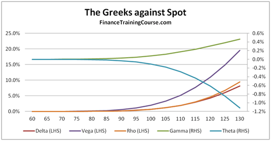
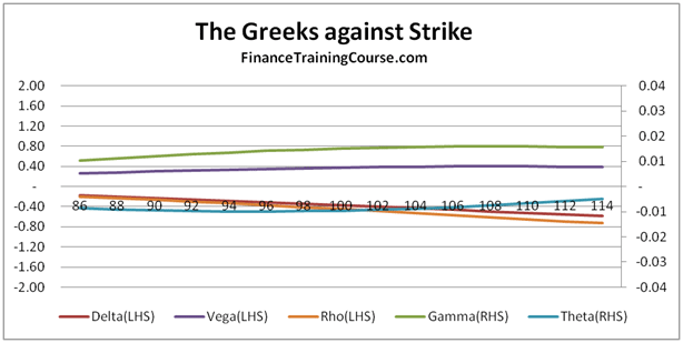
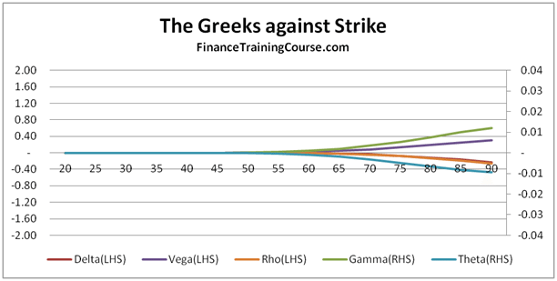
Figure 8 The Greeks against Spot. Deep out of money options
Figure 9 The Greeks against spot. AT, In and near money options
The next natural question deals with the valid range of values that Delta is expected to take. For a call option the range is between 0 and 1, as we have seen demonstrated above. Zero for deep out of money options, one for deep in money options. In between for all other shades.
For put options, Delta ranges between 0 and -1. Deep in money put options touch a Delta of -1, deep out of money put options reach a Delta of zero. The negative sign corresponds to a short position. To hedge a put, unlike a call, we short the underlying and invest the proceeds, rather than buy the underlying by borrowing the difference.
Sales and Trading Interview Guide: Dissecting Delta & Gamma – Against Strike
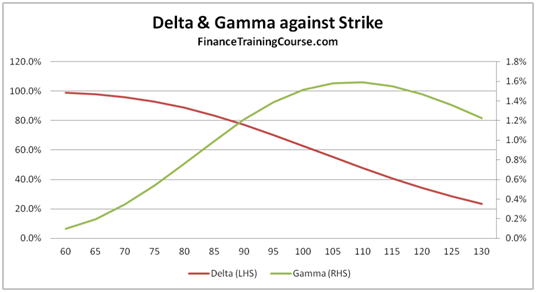
Figure 10 Delta & Gamma against changing strike price.
The next graph plots Delta and Gamma against changing strike price. We use a plot of both Delta and Gamma to reinforce the relationship between the two variables. Once again before you proceed further think about why do you see the two curves behave the way they do?
As the strike price moves to the right, the option gets deeper and deeper out of money. As it gets deeper in the deep out territory, the probability of its exercise and the amount required to hedge the exposure fall. Hence the steady decline in Delta as the strike price moves beyond the current spot price.
As the rate of change of Delta increases, we see Gamma rise by a proportionate amount. Gamma will only flatten out once the rate of change of Delta flattens out in the image above.
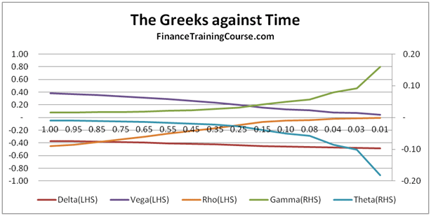
Sales and Trading Interview Guide: Dissecting Delta & Gamma – Against Time
The next three plots show how Delta and Gamma change as we vary time to expiry from a day to one year.
In the three snapshots that follow below, time moves from right to left (more to less). Once again we use both Delta and Gamma to reinforce the relationship between the two factors.
The only other variation from the options above is that we are now looking at three different options. An at money Call (Spot = 100, Strike = 100), an in money call (Spot = 110, Strike = 100) and a deep out of money call (Spot = 100, Strike = 200).
Notice how delta declines with time for an at money call, but rises to 1 for an in money call. Beyond a certain cut off point, it also rises for a deep out of money call but not as much as our first two pairs.
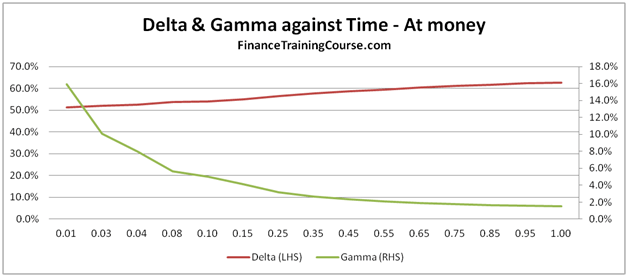
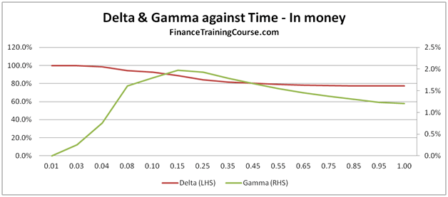
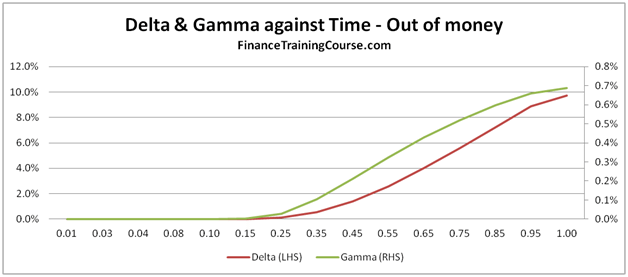
Figure 11 Delta & Gamm against Time for in, at and out of money options
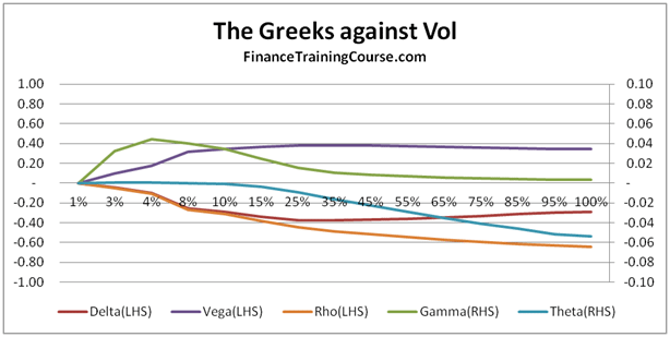
Sales and Trading Interview Guide: Dissecting Delta & Gamma – Against Volatility
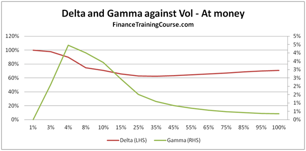
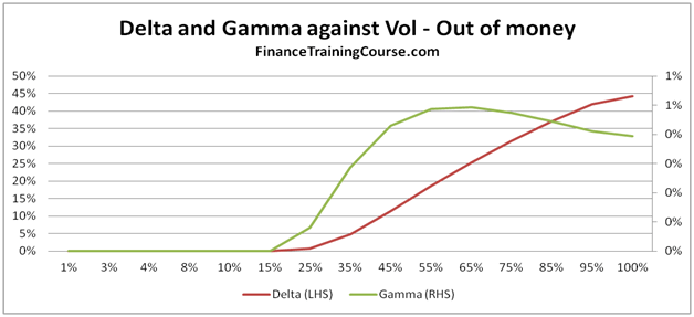
Figure 12 Delta, Gamma against Volatility. For at and out of money options.
For our last act, we plot Delta and Gamma against volatility and see a result which some students find counter intuitive.
For in, near or at money option, Delta actually falls with rising volatility. For most students this is a surprising result. Once would expect that with rising volatility, the value of the option should go up (correct) because the range of values reachable by the underlying is higher (also correct) hence leading to a higher probability of exercise (incorrect).
For deep out of money options, Delta rises with rising volatility. Gamma keeps pace initially but then runs out of steam as the rate of increase in Delta begins to flatten out.
To appreciate this behavior you actually have to move away from the Greeks and look at exercise probabilities.
Understanding the relationship between volatility, probability of exercise and price.
Our next three plots, show how the conditional probability of exercise N(d1), the unconditional probability of St > X, N(d1) and price behave and change for in, at and out of money European call options.
In the images beneath, Price is measured using the right hand scale, while the two probabilities are measured using the left hand scale.
For at, in and near money options, the two probabilities actually decline as volatility rise. Sounds counter intuitive when you consider that while the two probabilities are declining, the price of the option is actually rising.
Here is a hint, look up and think about volatility drag. For a deep out of money option the trend is reversed. Once again ask yourself why?
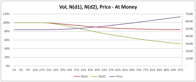
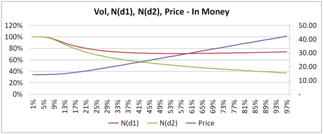
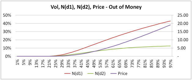
Figure 13 Vol, N(d1), N(d2) and Price for in, at, and deep out of money call options
Understanding Greeks: Option Delta and Gamma Review. Conclusion
If you are interested in a career on the floor or on a derivatives trading desk, you need to get very comfortable with the above graphs and behavior of Greeks across them. To the point of the lessons discussed becoming second nature – like riding a bike, breathing or drinking coffee. To remove the shock and awe caused by the partial differential equations behind the Greeks, we completely eliminated them from this post. In real life and when modeling them in excel you will have to get re-acquainted. Drop us a line with your questions or other dimensions that you would like us to address and if we can, we will do a few more posts on this topic.
Enjoy.
No related posts.
Sales and Trading Interview Guide: Understanding Greeks – Preface


Sales and Trading Interview Guide: Understanding Greeks
Trading requires a combination of intuition, discipline and process. Of the three intuition is the most difficult to teach, since discipline and process is an incentives and control game. While individual intuition can be built over years of experience there are rules that make it easier to pick up that intuition faster.
Institutional intuition gets passed on between generation of traders through shadowing, standards, processes and controls. This passage of rites becomes easier if you have a knack for the subject, if you already know some of the rules or if you are familiar with the trading language.
The sales and trading language has many dimensions dealing with execution, trading strategy, customer behavior and product variations. This book only focuses on one very limited aspect of that language – the aspect dealing with risk management, hedging and Greeks.
The challenge with this part of the language lies partly with the terminology (a range of Greek symbols), partly with the presentation (partial differential equation), with calculations (a combination of Greek symbols and partial differential equations) and with interpretation (can you please say that again in a language that we can all understand).
Most business school derivative courses run out of time before the product universe has been covered, let alone spend time on teaching how to read, predict or forecast the behavior of exotic Greek symbols. .
Advance derivative courses cover pricing and if we are lucky spend limited time on sensitivities and Greeks because of conflicts with other topics in the outline. Sometime as business school students all we get are case notes and text references that are long on definitions and calculations but short on guidance and practical applications.
Which is unfortunate because the option price sensitivity topic is difficult to grasp for most audiences given its very non-linear nature. It takes time to think comfortably in the non-linear world. We understand simple straight forward, single dimensional relationships very well. When you ask us to envision a new dimension or even worse collate reactions from multiple dimensions into a single trading decision, our mental frameworks breakdown.
To develop an appreciation for this topic you need at least a few days of hands on or modeling experience followed by active application of the same concepts. The reason why you have purchased this book is because you don’t have a few days. You possibly have a few hours or a night before that interview or presentation is due.
So we have tried to compress primary lessons into short bite sized pieces. There are some equations but we don’t spend time on them or their derivations. We do spend time on ground rules, behavior and intuition. As a trader I am more likely to ask you about how Gamma is going to behave under a given scenario and how that is different from Vega’s reaction.
Our assumption is that you have some familiarity with Options, Black Scholes and the derivative pricing world. If this is not the case you need more help which is available on our partially free site at FinanceTrainingCourse.com
This book is based on a four part MBA course on derivative pricing and risk management that I have taught in Dubai and Singapore and the risk and treasury management practice I have run since 2003. The material is based on training tools we developed to teach advance treasury concepts to our students using our signature hands on, equations off mode.
And now let’s go waltz with some Greek symbols.
Related posts:
The Sales and Trading Interview Guide Series – Understanding Greeks and Delta Hedging – Coming soon to an iPad near you…
Preparing for the quantitative portion of a sales and trading interview for a main street bank is a nightmare. Specially if the bank is an active derivative trader and wants it intake class of interns and full time analysts and associates to hit the Sales and Trading desk running.
While basic option concepts generally get covered quite well in the MBA curriculum, when it comes to option price sensitivities and Greeks, our understanding remains rudimentary and superficial. One reason is the focus on formulas and calculation rather than intuition and understanding. Most courses have run out of time when it comes to delta, gamma, vega, theta and rho and stop after a basic rudimentary coverage of the material.
There is a lot of good material available on basic quantitative and numerical techniques tested in a Sales and Trading interview. But when it comes to option price sensitivities or Greeks, available material generally looks like this.
As part of the work we do with customers and students, our Apple iPad iBooks team is working on two very interesting and exciting titles.
The first is the Sales and Trading Interview Guide – Understanding Greeks for Dummies. Using the interactive iBook template we will help you master your Greeks to such a level where future mention of delta, gamma, vega, theta and rho would no longer break you out in cold sweat and palpitations. The iBook will cover Greeks behavior across time, volatility, spot and strike prices using easy to understand language, graphs and self assessment quizes.
But it’s the second iPad iBook title that we are really excited about. Sales and Trading Interview Guide – Delta Hedging and other higher dimensions, will help you build your own delta hedging sheet in excel using Monte Carlo Simulation. Both iPads books will have options for purchasing supporting excel spread sheets that extend the concepts covered in the iBook.
Planned for release in mid September, the two books will increase our inventory of interactive iBook for iPad titles to 5. Please feel free to drop me a note if you would like to learn more about the release dates and table of content for both titles.
Related posts: