Convexity & Duration calculator for US Treasury Bills, Notes and Bonds. To demonstrate how Duration and Convexity are calculated for specific US Treasuries we select instruments from recent US Treasury bill, note and bond auctions. Please note that we are determining these metrics (Convexity & Duration) at issue. We will calculate Macaulay, Modified and Effective Duration […]
Tag: Fixed Income Portfolio
Practice Exam Test Question: Pricing and MTM of Interest Rate Swaps (IRS) – Partial solution
Practice Exam Test Question – Pricing and MTM of Interest Rate Swaps (IRS)
And now for the last and final part of our Practice Exam Test Question series on Pricing Interest Rate Swaps (IRS). In our first post we walked through the process of building a annualized forward curve and then extending it to semiannual rates.
In this post we will take the forward curve generated in the previous post and use it answer our Interest Rate Swaps (swap rate) and mark to market (valuation) questions.
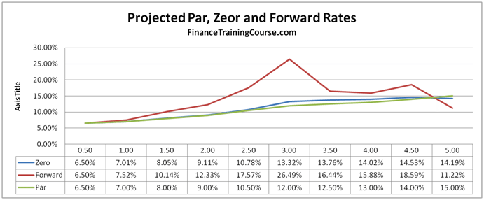
Here is the projected zero and forward rates curve from our previous post, posted here for convenience. Before you proceed further please take a quick look at the interest rate swap pricing free study guide to review our approach and methodology.

Mark to Market and Valuing an Interest Rate Swap – Practice Test Question and Partial solution
A client has recently entered into a 4.5 year floating rate loan for US$ 400,000,000? The loan will be effective six months from now and will use the following repayment schedule.
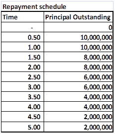
Figure 1 Practice Exam Question – Notional Principal for pricing Interest Rate Swaps
The client has asked for a quote for the an effective interest rate risk hedge that would offset the risk of rising interest rates.
a)
What would be the swap rate at cost or breakeven basis for this structure?
b) Would the client be paying fixed or receiving fixed
c) What would be the swap rate if the loan starts at time 2.5 with 10,000,000 and ends at time 3 with an outstanding principal of 10 million.
Here is the output from our solution Excel Sheet. The approach is as per interest rate swap pricing free study guide. The projected forward rates are as per the results above and were driven in the projected forward rates using bootstrapping post. As you can see that the trick here was recognizing that we didn’t have a normal interest rate swap but a forward starting amortizing swap and then adjust the pricing approach accordingly.
a) The exact breakeven swap rate is 13.718% and the breakeven value of each leg (fixed and floating) is 3.001609
million.
b) Since the client is hedging a floating rate loan with this swap he will be paying a fixed rate and receiving the floating rate or simply paying fixed.
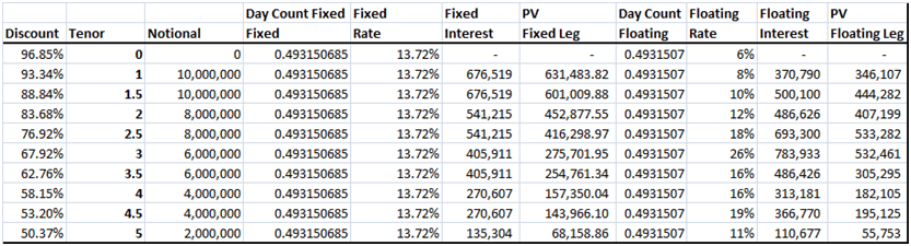
Figure 2 The practice test question solution – the interest rate swap pricing, MTM and valuation grid
c) This question is asking you to price a one step FRA or a Forward Rate Agreement. To solve it you should pick the row corresponding to tenor 2.5 and solve for a fixed rate that allows the present value of fixed and floating payments to completely offset each other. This fixed rate is 17.5732%. If you understood the question intuitively you should be able to answer it without resorting to the below solution by simply looking at the applicable forward rate and using that as the breakeven rate.

Figure 3 The practice test question – the FRA pricing, MTM and valuation grid
Common Interest Rate Swap pricing and valuation mistakes made by students in this question
- Not making the forward pricing adjustment for the forward starting interest rate swap
- Not using the correct notional amount. A number of students used a flat value of 400 million rather than the amortization schedule shared with the question above. Use the correct amortization schedule
- Not adjusting for the day count in the fixed as well as floating cash flows. Students often use the full rate when calculating semiannual payment, where as they should be using 180/360 or 182/365 * the relevant interest to account for the fact that the payment is a semiannual interest payment.
- Not using the correct applicable floating (forward rate)
d) Six month later the interest rates term structure has changed as shown below. Taking the original Swap structure and assuming that the Swap was purchased at the original breakeven Swap rate, what is the MTM (Mark to Market value of the Swap).
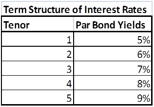
Figure 4 Practice Exam question – Revised Interest Rate Yield Curve
This question requires a simple re-application of the above process one more time. Here are the revised projected forward rates
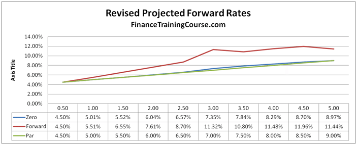
Figure 5 Revised projected forward rates
The trick now is to remember that we have all moved 6 months forward in time and the IRS is effective now. Based on this assumption this is how the revised grid looks like. The IRS has a negative MTM because we had expected rates to go up and they have actually come down.
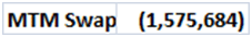
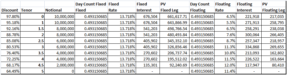
Figure 6 Pricing, MTM, Valuing the IRS under the new term structure and yield curve
Once again the biggest mistake students made here was not moving forward in time and pricing the IRS on an as is basis. The second biggest mistake was not using the updated curve and the old Swap Rate calculated from the earlier part of the question.
Related posts:
Practice Test Exam Question and Solution – Bootstrapping Zero and Forward Curves Case Study
Practice Test Exam Question Solution for Pricing Interest Rate Swaps – MBA course Derivatives I & II
Here is abbreviated partial solved solution to the practice exam question posed earlier. The practice exam question was used in Derivatives Pricing course taught to MBA students earlier in August 2012. The solution is presented in two parts. The first part of the solution focuses on the bootstrapping zero and forward curve part of the exam. The second part of the solution walks through the actual IRS pricing exercise. This post covers the first partial solution.
The practice exam question had three parts and hence the solution to the practice test question will also be presented in three parts. Before you proceed further please take a quick look at our free interest rate swaps pricing guide. We will only present the basic outputs from the solved solution sheet. You will need to review the interest rate swaps pricing study note to actually build the sheet yourself on your laptop.
Practice Test Exam Question Solution – A review of solution approach
Practice Test Part I dealt with build and plotting Zero and Forward curve using the data given and the bootstrapping approach applied on the given interest rate yield curve given below. The original yield curve was a 5 step curve that gave 5 annualized rates for 5 years.
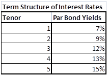
Figure 1 Practice Exam Question – Given Interest Rate Yield Curve
Practice Test Part II dealt with using the given zero and forward curves to price an Interest Rate Swap (IRS) and calculate the swap rate. The trick was extending the original curve to the new 10 step, semi annual yield curve implied by the 10 step notional amortization schedule given below.

Figure 2 Practice Test Question – The notional amortization schedule
Practice Test Part III dealt with marking to market (MTMing) the interest rate swap for an updated curve a few months later. Once again the trick is to extend the 5 step curve to a 10 step semi-annual curve which can then be used for pricing the interest rate swap.

Figure 3 Practice Test Question – the revised interest rate yield curve
Practice Test Exam Question Solution – Pricing Interest Rate Swap – Part I – Building the Forward Curve
The first step is to break the individual bonds down to their annual cash flows and treat each cash flow as an individual zero coupon bond as explained in the interest rate swap pricing study guide. The output from the first forward curve building step is shown below
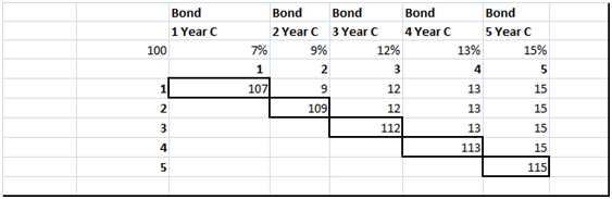
Figure 4 Practice Test Question – Solution – Breaking the bonds down to individual cash flows
The second step is to use the individual zero coupon cash flows to boot strap the present value of the principal cash flow at maturity for each of the par bonds as explained in the interest rate swap pricing study guide. The output from the boot strapping step is shown below.
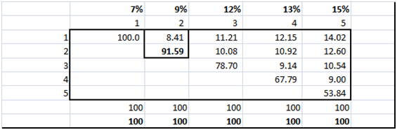
Figure 5 Practice Test Question – Bootstrapping discount factors
The third step is to apply the zero curve and forward curve formula to calculate the relevant zero and forward rates from the table above. As explained in the interest rate swap pricing study note. The output from the zero and forward rate calculation step is shown below.
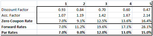
The final and forth step is to plot the Par, Forward and Zero rates in the required graphical format using MS Excel built in graphic tools.
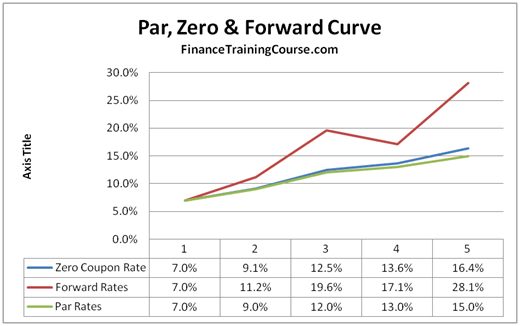
Figure 6 Practice Test Question – Plot of Par, Zero and Forward curves
Most students make it to this stage without any incident. Some however apply the wrong formula and end up with inconsistent results. If you are not happy with the results just apply a simple calculation cross check. If you calculate the relevant accumulation factors for each given year using your calculated Par, Zero and Forward curves they should all result in the same values as shown below.
The Par Curve Accumulation factor was already calculated above. For the Zero curve the accumulation factor is (1 + zero rate) raised to (compounding period). The accumulation factor for the forward curve is a similarly recursive calculation. Calculate the accumulation factor using the forward curve for the first year. Then use that in your calculation for calculating the accumulation factor using the forward curve for the second year.
If you see a value in the error term row, you have made a mistake in the calculations above. Review and check them.
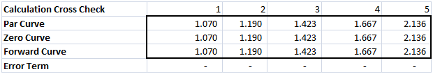
Figure 7 Practice Test Question – Calculation Cross Check
We have now successfully completed the first part of the test question. We now move on to part II.
Practice Test Exam Question Solution – Pricing Interest Rate Swap – Part II – Extending the Forward Curve
The second part of the question requires us to use the interest rate yield curve above to price a 10 step, semiannual interest rate swap. And this is where confusion reigned supreme.
Step One – Interpolated semiannual yields
We first need to break the original annual yields to maturity down into interpolated semiannual yields as shown below
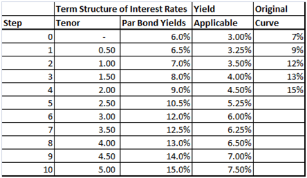
Figure 8 Practice Test Question – Interpolated semiannual yields.
Then using the same sequence of steps above we break the new implied semiannual bonds down to their zero coupon components, boot strap the curve, calculate the rates and plot the graphs.
Step Two – Zero Coupon Bonds
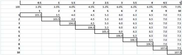
Figure 9 Practice Test Question – Zero Coupon Bonds by tenor
Step Three – Bootstrapped Discounted Cash Flows for Zeros
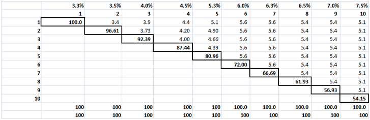
Figure 10 Practice Test Question – Bootstrapped Discounted Cash Flows
Step Four – Periodic and Annualized Par, Zero and Forward Rates
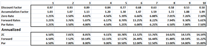
Figure 11 Practice Test Question – Model Output – Par, Zero and Forward Rates
Common Mistakes in Part II of the Test Exam
The most common mistakes that killed points for students in the second part of the practice test and exam questions were:
a) Not calculating the interpolated semiannual yields and using the original 5 annualized yield to price the 10 step interest rate swap
b) As a result of (a) above building a 5 x 5 or a 5 x 10 grid versus a 10 x 10 grid as shows in step two and step three above
c) Using annual rates rather than period rates in the 5 x 10 and 10 x 10 grid. Periodic rates are annualized rates divided by 2 since the coupon on the underlying loan is paid semi annually
d) Using periodic rates but then not annualizing them before using them in the IRS pricing later on in Part III of the practice test exam.
The correct solution and required graphical presentation if you didn’t suffer from mistake (a), (b), (c) and (d) above would look like this:
We continue our coverage of this exam question in our next post.
Pricing Interest Rate Swaps – The actual Final Exam question in full
Here is the original post that presented the question earlier today.
I teach the Derivative Pricing and Risk Management courses to EMBA and MBA students in Dubai and Singapore. In a recent exam one question caused a lot of heart ache and pain in exam takers. While most student understood the gist of the question, they still made a number of small mistakes that cost them valuable points in the final score.
If you have an interest rate swap pricing exam or test coming up, here is the solved solution that you can use as a practice exam or practice test question. For best results, first try the exam and the practice and test question and then work through the solution. Best of luck.
Pricing Interest Rate Swaps – Practice Exam – Test prep question
You are given the following term structure of interest rates for US$ using Yield to Maturity (YTM) of Par bonds that pay interest on a semi-annual basis

Figure 12 Test Prep – Practice Exam – The Interest Rates Yield Curve
Using these Par Bond Yields please answer the following questions:
7. Plot the following graph shown in Figure 1 using the above term structure and assuming that that coupon/interest is paid on a Semi Annual basis. This implies that you would need to build a 10 x 10 grid at semi-annual intervals for 5 years. Your graphical plot will show projected rates at 10 points at 10 half years. (15 Points)
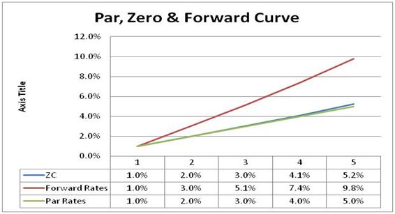
Figure 13 Practice Exam – Sample Par, Zero & Forward curve plot
Please see the next page for question number 8
8. A client has recently entered into a 4.5 year floating rate loan for US$ 400,000,000? The loan will be effective six months from now and will use the following repayment schedule. (35 points)

Figure 14 Practice Exam Question – Notional Principal for pricing Interest Rate Swaps
The client has asked for a quote for the an effective interest rate risk hedge that would offset the risk of rising interest rates.
a)
What would be the swap rate at cost or breakeven basis for this structure?
b) Would the client be paying fixed or receiving fixed
c) What would be the swap rate if the loan starts at time 2.5 with 10,000,000 and ends at time 3 with an outstanding principal of 10 million.
d) Six month later the interest rates term structure has changed as shown below. Taking the original Swap structure and assuming that the Swap was purchased at the original breakeven Swap rate, what is the MTM (Mark to Market value of the Swap).
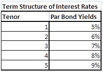
Figure 15 Practice Exam question – Revised Interest Rate Yield Curve
Related posts:
Pricing Interest Rate Swaps – Derivative pricing final exam question for practice exams & test prep
Pricing Interest Rate Swaps – Final Exam question for test prep
I teach the Derivative Pricing and Risk Management courses to EMBA and MBA students in Dubai and Singapore. In a recent exam one question caused a lot of heart ache and pain in exam takers. While most student understood the gist of the question, they still made a number of small mistakes that cost them valuable points in the final score.
If you have an interest rate swap pricing exam or test coming up, here is the sample question that you can use as a practice exam or practice test question. If you detailed hands on model building interviews for your Sales & Trading, FICC or Risk Management desks, the question has a few twists that can reveal how detail oriented and hands on your candidate is.
For best results, first try the exam and the practice and test question and then work through the solution (to be presented in the next post). Do the question under exam conditions and try and attempt the practice question in one sitting.
Best of luck for your exam.
Pricing Interest Rate Swaps – Practice Exam – Test prep question
You are given the following term structure of interest rates for US$ using Yield to Maturity (YTM) of Par bonds that pay interest on a semi-annual basis

Figure 1 Test Prep – Practice Exam – The Interest Rates Yield Curve
Using these Par Bond Yields please answer the following questions:
7. Plot the following graph shown in Figure 1 using the above term structure and assuming that that coupon/interest is paid on a Semi Annual basis. This implies that you would need to build a 10 x 10 grid at semi-annual intervals for 5 years. Your graphical plot will show projected rates at 10 points at 10 half years. (15 Points)

Figure 2 Practice Exam – Sample Par, Zero & Forward curve plot
Please see the next page for question number 8
8. A client has recently entered into a 4.5 year floating rate loan for US$ 400,000,000? The loan will be effective six months from now and will use the following repayment schedule. (35 points)

Figure 3 Practice Exam Question – Notional Principal for pricing Interest Rate Swaps
The client has asked for a quote for the an effective interest rate risk hedge that would offset the risk of rising interest rates.
a)
What would be the swap rate at cost or breakeven basis for this structure?
b) Would the client be paying fixed or receiving fixed
c) What would be the swap rate if the loan starts at time 2.5 with 10,000,000 and ends at time 3 with an outstanding principal of 10 million.
d) Six month later the interest rates term structure has changed as shown below. Taking the original Swap structure and assuming that the Swap was purchased at the original breakeven Swap rate, what is the MTM (Mark to Market value of the Swap).

Figure 4 Practice Exam question – Revised Interest Rate Yield Curve
Related posts:
Advance Risk Management Models – Workshop & Training reference page
Advance Risk Management Models – Free Online Resource Guide
Advance Risk Management Models (aka RM II) course is a 1 credit course taught at the SP Jain Campus in Dubai and Singapore by Jawwad Ahmed Farid.
A variation of this course was recently delivered (22-29th August 2012) at the SP Jain Dubai Campus by Jawwad. A smaller version of the course is scheduled for delivery at the Singapore campus in mid October 2012.
The course builds up on the work done in earlier MBA specialization courses (Risk Management I, Derivatives I and Derivatives II) conducted for regular and executive MBA students. The focus is on model building and practical applications using hands on models in Excel. The course reviews risk management models from the world of portfolio optimization, derivatives pricing and hedging, hedge optimization, banking regulation, credit risk, probability of default estimation.
Advance Risk Management Models – Course Prerequisites
Students are expected to be comfortable with materials covered in Risk Management I and the Derivatives I and II course series. See the reference site for Risk Management I for a quick review of risk management concepts. Without the relevant background you are likely to struggle so familiarity with the shared material is highly recommended.
Advance Risk Management Models – Course Plan
Here is the lesson plan for seven days of classes. The training workshop classes run for 150 minutes every day with homework assignments due for submission the next morning. As course material is documented and available for release the core theme links on this page (below) will be updated.
Advance Risk Management Models – Core Themes and study notes
- Fixed Income Value at Risk (VaR) Calculations for fixed rate bonds
- Fixed Income Investments Portfolio Optimization Model using Excel Solver
- Implied volatility, a simple introduction
- Delta Hedging introduction
- Delta Hedging European Calls and Put Contracts using Monte Carlo Simulation
- Option Greek Crash Course – Delta, Gamma, Vega, Theta & Rho
- A review of bank regulation and why it really doesn’t work.
- Basic credit analysis and models
- Probability of default calculations using the structured (Merton’s) approach
- Kill a bank in one day simulation – integrating funding, liquidity, ALM, credit allocation, capital adequacy and probabilty of shortfall.
Course note in the form of html posts are available for free. Downloadable pdf files and excel templates are available for purchase separately from our online store.
Related posts:
- Fixed Income Investment Portfolio Management & Optimization Case Study – Risk Training
- Financial Risk Management Workshop – Value at Risk, Volatility and Trailing correlations – Day One
- The Asset Liability and Liquidity Management Training Workshop, Subang Holiday Resort, Kula Lumpur, Malaysia, January 2011.
Fixed Income Investment Portfolio Management & Optimization Case Study – Risk Training
Fixed Income Investment Portfolio Management using duration, convexity and Excel solver
It doesn’t matter if you manage a pension fund, a life insurance trust fund or the proprietary book of an investment bank, at some point in time you hit your allocation and risk limits and need to rebalance your portfolio.
In most instances your limits and target accounts focus on interest rate sensitivity, volatility, Yield to risk ratios, liquidity and concentration limits. Your objective is to create the most efficient fixed income investment portfolio that balances an optimal mix of the above constraints against yield to maturity. The time tested, risk versus reward tweak.
In our new risk training workshop for fixed income portfolios case study we will build a simple model using Excel solver that shows how to handle the fixed income portfolio optimization problem. The model can be easily extended to handle larger portfolios and additional constraints around liquidity, factor sensitivity, volume concentration, value at risk and volatility.
For the purpose of this case study we will assume that we are advising a large pension fund who is re-evaluating fixed income portfolio allocation due to its new investment policy. The assets under management at the fund are US$500 million. We want to recommend:
- Portfolio allocation that minimizes duration
- Portfolio allocation that maximizes convexity
The liabilities are also equal to $500 million with a weighted average maturity of 20 years. Modified duration or interest rate sensitivity of liabilities was last measured in the monthly risk report at 9%.
Fixed Income Portfolio Management: Introducing Duration and Convexity
Duration is a measure of how prices of interest sensitive securities change as the underlying rate of interest changes. For example, if duration of a security works out to 2 this means roughly that for a 1% increase in interest rates price of the instrument will decrease by 2%. Similarly, if interest rates were to decrease by 1% the price of the security would rise by 2%.
Here is the numerical approximation for modified duration.
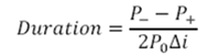
Figure 1 Fixed Income Portfolio management. Numerical approximation for duration
Convexity: The Duration approximation of change in price due to changes in the yield works only for small changes. For larger changes there will be a significant error term between the actual price change and that estimated change using duration.
Convexity improves on this approximation by taking into account the curvature of the price/ yield relationship as well as the direction of the change in yield. By doing so it explains the change in price that is not explained by Duration.
A positive convexity measure indicates a greater price increase when interest rates fall by a given percentage relative to the price decline if interest rates were to rise by that same percentage. A negative convexity measure indicates that the price decline will be greater than the price gain for the same percentage change in yield.
Duration and Convexity together are used to immunize a portfolio of assets and liability against interest rate shock.
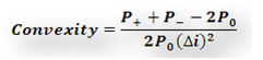
Figure 2 Fixed Income Portfolio Management. Numerical approximation for Convexity
Fixed Income Portfolio Management: Introducing the Optimization model
Our first scenario assumes a rising interest rate outlook. Ignoring liabilities and maturity mismatch for now, our fund manager would like to rebalance the portfolio to minimize duration so that the value of assets do not fall significantly due to changes in interest rates. We assume:
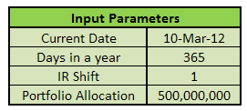
Figure 3 – Fixed Income Investment Portfolio – Date, Rate shift, size.
Fixed Income Investment Portfolio Management: Breaking down the optimization model
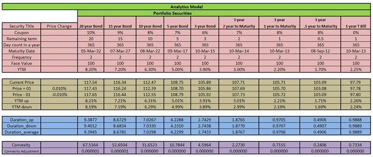
Figure 2 – Fixed Income Investment Portfolio Management: The securities analytics model
There are four parts to this model:
- Part 1- The securities universe specification: This is the pink-shaded area and defines the complete investment universe. You can only allocate a security if it is described in universe. Assets are classified in buckets of 20, 15, 10, 5 and 3 year maturities. We have assumed that current date (the valuation date) is the same as date of purchase (the settlement or value date) for all assets in all buckets.
-
Part 2 – The securities pricing model: This calculates the price and yield and is shaded brown. Current price is calculated using the Excel price function as illustrated below:
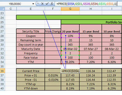
Figure 3 – Price calculation
The excel price (bond pricing) function is based on the data inputs of settlement date, date of maturity, coupon rate, yield to maturity, frequency and basis. Frequency here is 2 which mean that coupons are paid semi-annually. Cell $D$4 is the current date used in the input parameters in Figure 1.
Price changes just add or subtract the specified interest rate shocks and recalculate new prices for use in duration and convexity calculations. The rate shocks are 1 basis points (1/10,000).
-
Part 3 – Portfolio Duration Calculation: this is shaded blue and shows duration calculations. Duration is calculated using the duration approximation formula introduced above:

Figure 4 Fixed Income Investment Portfolio: Duration approximation
In the context of the Analytics Model, this is calculated as follows:
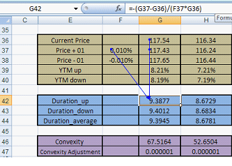
Figure 4 – Duration calculation
In calculation of Duration-down, Cell G44 is replaced by G45 and F44 is replaced by F45. Note that the general form of the formula is applied but instead of just calculating duration in one line, duration up and down are calculated respectively and the average of both is taken.
This average of the two durations will be used in our model. - Part 4 – Portfolio Convexity Calculation
-
The final part of the model calculates convexity and is highlighted in purple. The applicable convexity formula is:
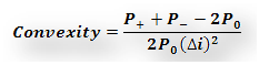
Figure 5 Fixed Income Portfolio Investment – Convexity calculation
The calculation is as under:
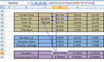
Figure 5 – Convexity calculation
The convexity adjustment is calculated using the formula:
Fixed Income Investment Portfolio Management: Summarized Portfolio Analytics
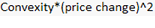
We now need a summarized portfolio analytics table that can be used in our optimization process. The results derived by combining the actual portfolio allocation and the portfolio analytics generated above would appear as shown below:
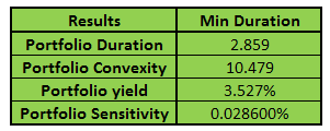
Figure 6 – Fixed Income Investment portfolio management. Portfolio analytics results
How are these results calculated? The answer is through the Analytics Model and the allocation of assets followed currently for each bucket. The allocation table is shown below:

Figure 7 – Portfolio allocation
Notice that the total bond portfolio allocation is 97% not 100%. 3% of the allocation is held in cash and/or non-interest sensitive securities.
Portfolio Duration is calculated by using the Excel sum-product function.
Sum-product is simply the combination of two operation that involves multiplying the individual cells in two vectors (Portfolio Allocation, Security Duration) and then summing the resulting product across all cells.
For instance (10%*duration average for 15 year bond) + (10%*duration average for 10 year bond)….. And so on.
Portfolio Convexity is calculated in the same manner by using the Excel sum-product function. (10%*convexity for 15 year bond) + (10%*convexity for 10 year bond)….. And so on.
And ditto for portfolio yield calculations. (10%*portfolio yield for 15 year bond) + (10%*portfolio yield for 10 year bond)….. And so on.
Figure 8 – Fixed Income Investment Portfolio Management: Calculating portfolio yield, portfolio duration and portfolio convexity
Portfolio sensitivity of -0.028600% is calculated in the following way:
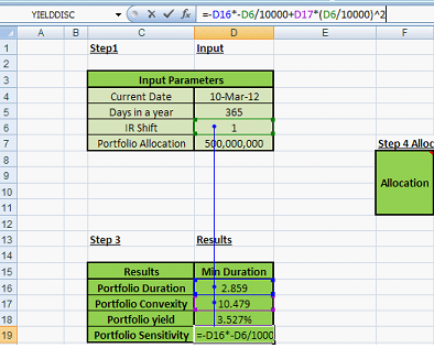
Figure 9 – Fixed Income Investments Portfolio Management. Calculating portfolio sensitivity
IR shift is the interest rate shift. It is measured in bps (basis point shift).
Fixed Income Investments Portfolio Management: Portfolio Optimization using solver
If we had a single linear equation representing a single constraint and a single position, the Excel Goal seek function would be sufficient. However a multi position fixed income investment portfolio has many constraints and many positions. In addition because you are dealing with bonds, the underlying model is no longer linear. You need a non-linear tweak to make it work.
The Excel solver function helps us optimize our portfolio allocation model with a few tweaks. We demonstrate the simplest of scenario in this write up but they can very easily be extended. As is the case with all optimization models, the trick is in designing the constraints. While there can be only one objective function (minimize or maximize a specific portfolio metric), with the right constraint design you could get close to a near optimal solution reasonably quickly. While the current model focuses only on fixed income investment portfolio, the design of the model can very easily be extended to multi-class portfolios. In addition new target accounts and risk constraints can be added just as easily.
Fixed Income Investments Portfolio Optimization. Optimizing the base case – Minimizing duration
The trustees of our pension fund have given a target to the investment fund manager to earn at least 3%. Bond proportion should be 99% of the fund, with the remaining for cash. Risk management and diversification targets specify that no greater than 13% of the total fund be allocated to any given asset bucket.
Given these objectives, how should the investment manager set out to minimize duration?
The targets are effectively constraints. Once we have defined them correctly, the solver function takes these constraints into account, evaluates the target optimization cell (minimize duration), and searches for an optimal solution. Since the layout of the spreadsheet has been described above, all we know need to do is to define the solver model and click solve.
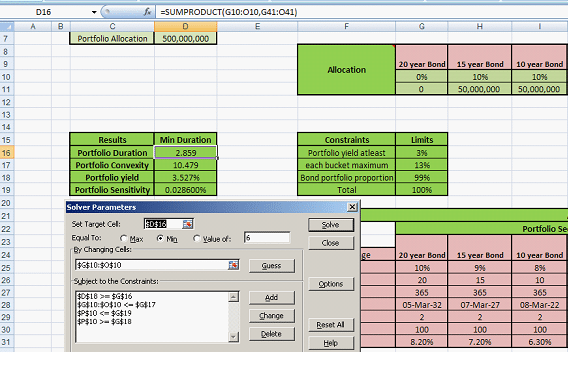
Figure 10 – Fixed Income Investments Portfolio Management. Using Excel Solver for minimizing duration for a fixed income portfolio
Pick ‘Min’ as your objective and then click ‘Solve’. Solver will work through the model till it reaches the optimal solution. The revised fixed income portfolio allocation is as follows:
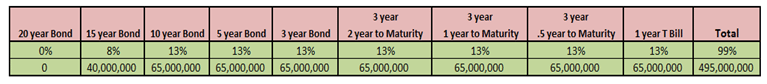
Figure 11 – Portfolio allocation
Note that none of the asset bucket has higher than 13% proportion of assets. Also 99% is invested in bonds, rest in cash. The revised portfolio analytics summarizing our target account is also shown below:
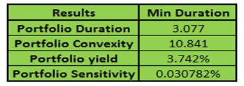
Figure 12 – Fixed income investments portfolio management – Revised portfolio analytics
Fixed Income Investments Portfolio Optimization – Maximizing Convexity
Positive convexity is generally a desirable attribute in a portfolio. In addition to minimizing duration, an alternate case could be made for maximizing convexity. If you expect rates to decline, a more convex fixed rate asset would rise by more compared to a less convex asset.
All it will take is set the Target Cell at portfolio convexity instead of duration. Note that in solver we click on ‘max’ instead of ‘min’ this time. The revised allocation is as follows:

Figure 13 – Fixed Income Investments Portfolio Management – Revised optimal portfolio allocation for maximizing convexity
And the revised portfolio analytics results for both the maximized convexity and minimized duration scenarios are presented below:
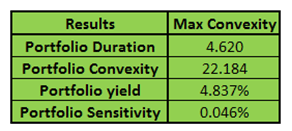
Figure 14 – Fixed Income Investment Portfolio Management – Optimized portfolio analytics results
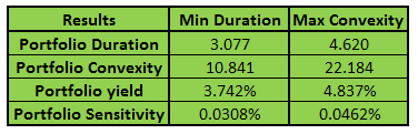
Figure 15 – Fixed Income Investments Portfolio Management – Consolidated results
Fixed Income Investments Portfolio Optimization. Next steps
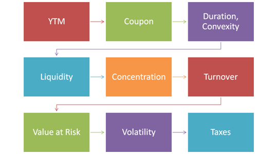
You can easily extend the model to include constraints for value at risk, volatility, interest rate mismatch, gap management, concentration, portfolio liquidity, daily, monthly and weekly turnover, credit ratings and grades. A sample sheet showcasing some of these variations will be available for sale early next week at our store.
If you need more help beyond the sample portfolio, we also help customer build customized portfolio builds and solver models.
Related posts: